


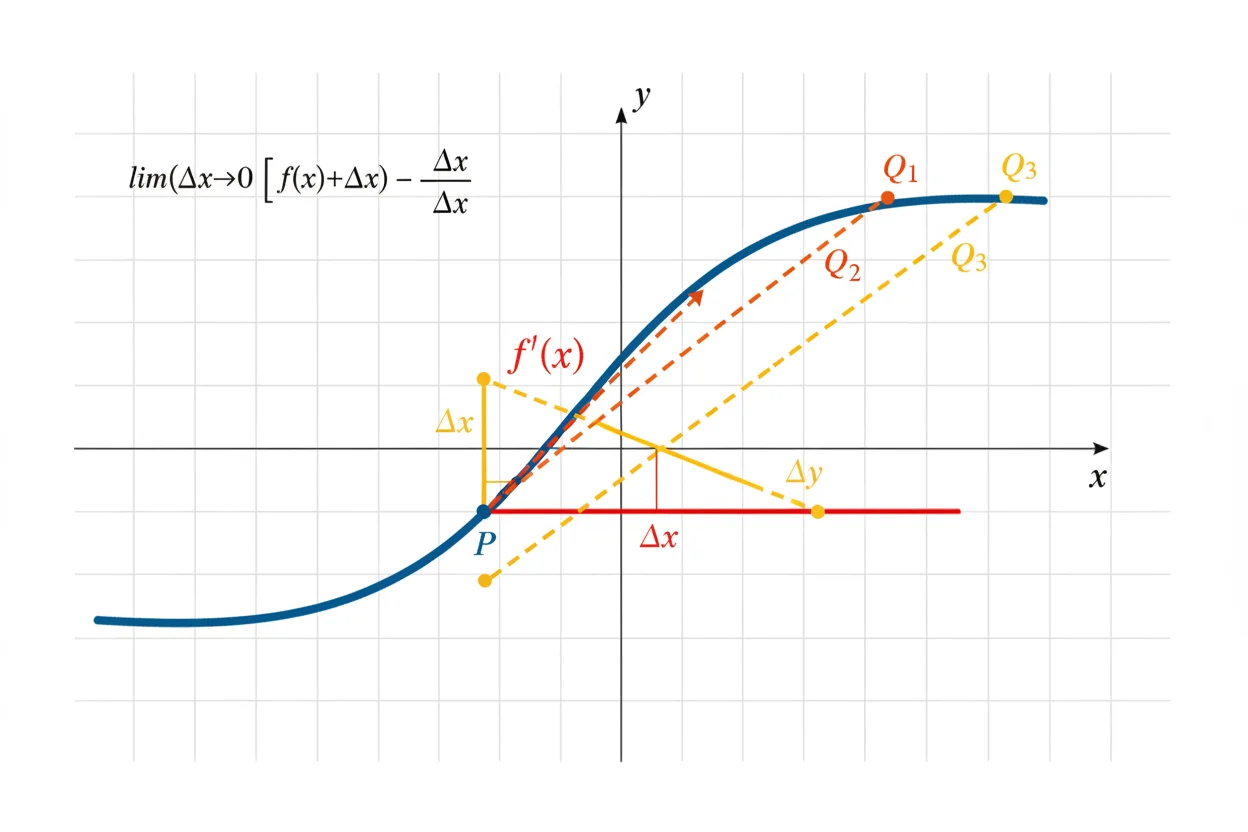
A derivative measures how quickly a function changes with respect to its input. Geometrically, the derivative at a point is the slope of the tangent line to the graph at that point. In an applied setting, it can represent an instantaneous rate such as velocity, growth rate, marginal cost, temperature change, or another rate of change. The derivative of f(x) is commonly written as f′(x), dy/dx, or d/dx[f(x)]. Its formal definition comes from a limit of average rates of change over increasingly small intervals. Basic functions can often be differentiated directly using standard rules, while products, quotients, and composite functions require specialized differentiation rules. A derivative can be positive, negative, zero, or undefined depending on the local behavior of the function. Understanding both its calculation and interpretation is essential because derivatives connect function behavior with slopes, rates, extrema, approximation, and later calculus methods.
What Is a Derivative?
For a function:
y = f(x)
the derivative describes the instantaneous change in y produced by a change in x.
It can be written as:
f′(x)
or:
dy/dx
or:
d/dx[f(x)]
If:
f(x) = x²
then:
f′(x) = 2x
This tells us that the slope of y = x² depends on x.
At x = 3:
f′(3) = 2(3) = 6
So the tangent line to y = x² has slope 6 at x = 3.
The broader topic of derivatives includes related forms and applications, while the derivative itself expresses the instantaneous rate of change of a particular function.
Derivative Formula From First Principles
The formal derivative formula is:
f′(x) = lim [f(x + h) − f(x)]/h as h → 0
The expression:
[f(x + h) − f(x)]/h
calculates the average rate of change between two nearby points.
As:
h → 0
the second point approaches the first, and the secant-line slope approaches the tangent-line slope.
The limit exists only when the function has suitable local behavior at that point.
Understanding the Difference Quotient
The expression:
[f(x + h) − f(x)]/h
is called the difference quotient.
Its numerator measures change in output:
Δy = f(x + h) − f(x)
Its denominator measures change in input:
Δx = h
So it has the familiar rate form:
change in output / change in input
Before taking the limit, this is an average rate of change. After taking the limit as h approaches zero, it becomes an instantaneous rate of change.
Finding a Derivative From First Principles
Consider:
f(x) = x²
Start with:
f′(x) = lim [f(x + h) − f(x)]/h as h → 0
Calculate:
f(x + h) = (x + h)²
Expand:
(x + h)² = x² + 2xh + h²
Substitute:
f′(x) = lim [(x² + 2xh + h²) − x²]/h as h → 0
Simplify:
f′(x) = lim (2xh + h²)/h as h → 0
Factor h:
f′(x) = lim h(2x + h)/h as h → 0
For h ≠ 0, cancel h:
f′(x) = lim (2x + h) as h → 0
Therefore:
f′(x) = 2x
The derivative of x² is:
2x
Derivative at a Specific Point
There is a distinction between finding a derivative function and evaluating a derivative at one point.
If:
f(x) = x³
then:
f′(x) = 3x²
This is the derivative function.
At x = 2:
f′(2) = 3(2²)
= 12
So the instantaneous slope at x = 2 is 12.
Derivative as the Slope of a Tangent Line
Suppose a graph has equation:
y = f(x)
At x = a, the tangent-line slope is:
m = f′(a)
Once the derivative is known, the tangent line through:
(a, f(a))
can be written using point-slope form:
y − f(a) = f′(a)(x − a)
For example, take:
f(x) = x²
at:
x = 2
Then:
f(2) = 4
and:
f′(x) = 2x
so:
f′(2) = 4
The tangent line is:
y − 4 = 4(x − 2)
Simplify:
y = 4x − 4
Derivative as an Instantaneous Rate of Change
Suppose position is given by:
s(t) = t² + 3t
where s is measured in meters and t in seconds.
Differentiate:
s′(t) = 2t + 3
Because the derivative of position with respect to time is velocity:
v(t) = 2t + 3
At t = 4:
v(4) = 2(4) + 3
= 11
The instantaneous velocity is:
11 m/s
This interpretation explains why derivatives are widely used whenever one quantity changes continuously with another.
Constant Rule
The derivative of a constant is zero.
d/dx[c] = 0
For example:
f(x) = 9
Then:
f′(x) = 0
A constant function has a horizontal graph, so its slope is zero everywhere.
Constant Multiple Rule
If c is a constant:
d/dx[c f(x)] = c f′(x)
For example:
f(x) = 5x³
Differentiate:
f′(x) = 5(3x²)
= 15x²
Sum and Difference Rules
Differentiation distributes across sums and differences.
d/dx[f(x) + g(x)] = f′(x) + g′(x)
and:
d/dx[f(x) − g(x)] = f′(x) − g′(x)
For example:
f(x) = x³ + 4x² − 7x + 6
Differentiate term by term:
f′(x) = 3x² + 8x − 7
The constant 6 disappears because its derivative is zero.
Power Rule
For:
f(x) = xⁿ
the standard power rule is:
d/dx[xⁿ] = nxⁿ⁻¹
For example:
f(x) = x⁵
Then:
f′(x) = 5x⁴
If:
g(x) = x⁻²
then:
g′(x) = −2x⁻³
= −2/x³
The power rule makes many elementary derivative calculations immediate.
Example: Differentiate a Polynomial
Differentiate:
f(x) = 4x⁵ − 3x³ + 6x − 8
Apply the derivative to each term:
d/dx[4x⁵] = 20x⁴
d/dx[−3x³] = −9x²
d/dx[6x] = 6
d/dx[−8] = 0
Therefore:
f′(x) = 20x⁴ − 9x² + 6
Product of Two Functions
When two nonconstant functions are multiplied, differentiating each factor separately and multiplying the answers is generally incorrect.
For:
y = f(x)g(x)
the product rule is:
y′ = f′(x)g(x) + f(x)g′(x)
Consider:
y = x²(x³ + 1)
Using the product rule:
y′ = 2x(x³ + 1) + x²(3x²)
Simplify:
y′ = 2x⁴ + 2x + 3x⁴
y′ = 5x⁴ + 2x
Expanding the original expression first gives the same result:
y = x⁵ + x²
y′ = 5x⁴ + 2x
Quotient of Two Functions
When one function is divided by another, the quotient rule can be used.
For:
y = f(x)/g(x)
with:
g(x) ≠ 0
the derivative is:
y′ = [g(x)f′(x) − f(x)g′(x)]/[g(x)]²
For example:
y = x²/(x + 1)
Let:
f(x) = x²
g(x) = x + 1
Then:
f′(x) = 2x
g′(x) = 1
So:
y′ = [(x + 1)(2x) − x²]/(x + 1)²
Simplify the numerator:
2x² + 2x − x²
= x² + 2x
Therefore:
y′ = (x² + 2x)/(x + 1)²
Composite Functions
A composite function contains one function inside another.
For example:
y = (x² + 1)⁵
The outer function is a fifth power, while the inner function is x² + 1.
The chain rule differentiates the outer function and multiplies by the derivative of the inner function:
y′ = 5(x² + 1)⁴(2x)
Therefore:
y′ = 10x(x² + 1)⁴
Recognizing composition is essential because applying only the outer derivative would omit the factor 2x.
Exponential Function Derivatives
For the natural exponential function:
f(x) = eˣ
the derivative is:
f′(x) = eˣ
The function is unusual because it equals its own derivative.
For a positive constant a:
d/dx[aˣ] = aˣ ln(a)
For example:
d/dx[2ˣ] = 2ˣ ln(2)
Logarithmic Derivatives
For:
f(x) = ln(x)
with x > 0:
f′(x) = 1/x
For example:
f(x) = 3ln(x)
Then:
f′(x) = 3/x
If a logarithm contains a nontrivial inner function, the chain rule is also required.
Trigonometric Derivatives
Several common trigonometric derivatives are:
d/dx[sin x] = cos x
d/dx[cos x] = −sin x
d/dx[tan x] = sec²x
For example:
f(x) = 4sin x − 2cos x
Then:
f′(x) = 4cos x + 2sin x
Angles are assumed to be measured in radians for these standard formulas.
Derivative and Continuity
Differentiability implies continuity at the same point.
In symbolic form:
differentiable at x = a ⇒ continuous at x = a
The reverse is not always true.
For example:
f(x) = |x|
is continuous at x = 0 but does not have an ordinary derivative there because the graph has a sharp corner.
From the left, the slope is:
−1
From the right, the slope is:
1
Because the one-sided slopes disagree, f′(0) does not exist.
When Does a Derivative Not Exist?
A derivative may fail to exist at several types of points.
A sharp corner is one example. A cusp can also cause the derivative to fail. A vertical tangent may produce an unbounded slope rather than a finite derivative. A discontinuity prevents ordinary differentiability altogether.
Consider:
f(x) = |x|
At x = 0:
left-hand slope = −1
right-hand slope = 1
Therefore:
f′(0) does not exist
A graph can therefore be defined and continuous at a point without being differentiable there.
Positive Derivative
If:
f′(x) > 0
throughout an interval, the function is increasing there.
For example:
f(x) = x²
has:
f′(x) = 2x
When:
x > 0
we have:
2x > 0
so x² is increasing on the positive side of the x-axis.
Negative Derivative
If:
f′(x) < 0
throughout an interval, the function is decreasing there.
For:
f(x) = −x²
we have:
f′(x) = −2x
When x > 0:
f′(x) < 0
so the function decreases on that interval.
Zero Derivative
If:
f′(a) = 0
the tangent line at x = a is horizontal.
Such points are important when studying possible local maxima and minima.
For example:
f(x) = x² − 4x + 7
Differentiate:
f′(x) = 2x − 4
Set the derivative equal to zero:
2x − 4 = 0
x = 2
At x = 2, the tangent is horizontal.
Problems that use derivatives to find the best, largest, smallest, cheapest, or most efficient value are studied systematically in optimization.
Derivative in Related Rates
Sometimes several changing quantities are connected by one equation.
For example, the area of a circle is:
A = πr²
If the radius changes with time, both A and r depend on t.
Differentiating with respect to time gives:
dA/dt = 2πr dr/dt
This connects the rate of change of area to the rate of change of radius.
Problems built around this structure are known as related rates problems.
Implicitly Defined Functions
Not every relationship is initially solved for y.
Consider:
x² + y² = 25
Differentiating both sides with respect to x gives:
2x + 2y(dy/dx) = 0
Solve for dy/dx:
2y(dy/dx) = −2x
dy/dx = −x/y
This process is called implicit differentiation and is useful when isolating y would be inconvenient or unnecessary.
Derivative and Differentials
If:
y = f(x)
then the differential dy is related to dx by:
dy = f′(x) dx
The derivative therefore acts as the local scaling factor connecting a small input change with the corresponding linearized output change.
The dedicated topic of differentials develops this notation and its use in approximation.
For sufficiently small changes:
Δy ≈ f′(x)Δx
This approximation is often accurate when Δx is small and the function behaves smoothly.
Derivative and Definite Integral
The derivative measures instantaneous change, while a definite integral accumulates change over an interval.
If F′(x) = f(x), then under the usual conditions:
∫ₐᵇ f(x) dx = F(b) − F(a)
This relationship allows differentiation and integration to function as inverse processes in fundamental calculus problems.
Derivative in Differential Equations
A differential equation contains an unknown function and one or more of its derivatives.
For example:
dy/dx = 3y
does not simply ask for the derivative of a known function. Instead, it asks which functions have a derivative equal to three times the original function.
Thus ordinary differentiation starts with a function and finds its derivative, while differential equations frequently start with derivative relationships and seek the function.
Partial Derivatives
For functions with more than one independent variable, the derivative concept extends to partial differentiation.
Suppose:
f(x, y) = x²y + 3y²
A partial derivative with respect to x treats y as constant:
∂f/∂x = 2xy
With respect to y:
∂f/∂y = x² + 6y
These are multivariable extensions of the same basic idea of measuring change.
Directional Change
In multiple dimensions, change can also be measured in a chosen direction rather than along only one coordinate axis.
The directional derivative measures that rate of change and builds on partial derivatives and vector methods.
This differs from a basic single-variable derivative, where there is only one independent input direction to consider.
Derivative Versus Cross Product
Both calculus and linear algebra use operations involving direction, but they should not be confused.
A derivative measures how a function changes. The cross product combines two three-dimensional vectors to produce a vector perpendicular to both.
They can appear together in advanced vector calculus, but they answer different mathematical questions.
The broader Calculus & Linear Algebra framework connects these ideas while preserving their individual roles.
Example: Find the Derivative and Evaluate It
Let:
f(x) = 2x³ − 5x² + 4x − 1
Differentiate:
f′(x) = 6x² − 10x + 4
Now find the derivative at x = 2:
f′(2) = 6(2²) − 10(2) + 4
= 24 − 20 + 4
= 8
Therefore:
f′(2) = 8
The graph of f has tangent slope 8 at x = 2.
Example: Derivative of a Radical
Consider:
f(x) = √x
Rewrite the radical:
f(x) = x¹ᐟ²
Apply the power rule:
f′(x) = (1/2)x⁻¹ᐟ²
Therefore:
f′(x) = 1/(2√x)
For real x > 0, this gives a finite derivative.
At x = 4:
f′(4) = 1/(2√4)
= 1/4
Example: Derivative of a Reciprocal
Consider:
f(x) = 1/x
Rewrite:
f(x) = x⁻¹
Differentiate:
f′(x) = −x⁻²
Therefore:
f′(x) = −1/x²
The derivative exists wherever:
x ≠ 0
At x = 0 the original function itself is undefined.
Example: Instantaneous Velocity
Suppose:
s(t) = 4t² − 2t + 7
Differentiate position to find velocity:
v(t) = s′(t)
v(t) = 8t − 2
At t = 3:
v(3) = 8(3) − 2
= 22
If s is measured in meters and t in seconds, the instantaneous velocity is:
22 m/s
Units of a Derivative
The units of a derivative are:
output units / input units
If distance is measured in kilometers and time in hours:
ds/dt
has units:
kilometers per hour
If cost C is measured in dollars and quantity q in units:
dC/dq
has units:
dollars per unit
Checking derivative units is a useful way to confirm an interpretation.
Common Mistakes
A common mistake is confusing the value of a function with the value of its derivative. If f(2) = 5, that does not imply f′(2) = 5.
Another frequent error is applying the power rule without reducing the exponent by one. For:
x⁵
the derivative is:
5x⁴
not 5x⁵.
Constants must also be handled correctly. The derivative of a constant is zero, while the derivative of cx is c.
Products and quotients of nonconstant functions require their own rules; simply differentiating each function independently and then multiplying or dividing the results generally gives the wrong answer.
Composite functions require the derivative of the inner function as well as the outer function.
Finally, a derivative should not automatically be assumed to exist. Corners, cusps, vertical tangents, discontinuities, and domain boundaries may require closer inspection.
Frequently Asked Questions
What is the formula for a derivative?
The first-principles definition is:
f′(x) = lim [f(x + h) − f(x)]/h as h → 0
when the limit exists.
What does a derivative mean?
A derivative measures instantaneous rate of change. Geometrically, it gives the slope of the tangent line to a function’s graph.
What does f′(x) mean?
It represents the derivative function of f(x). Its value at a specific input x gives the instantaneous rate of change at that point.
What is the derivative of a constant?
The derivative of any constant is zero:
d/dx[c] = 0
What is the derivative of x?
d/dx[x] = 1
because the graph y = x has constant slope 1.
What does a positive derivative mean?
A positive derivative indicates that the function is increasing locally as x increases.
What does a negative derivative mean?
A negative derivative indicates that the function is decreasing locally.
What does a zero derivative mean?
A zero derivative means the tangent line is horizontal at that point. It may indicate a local maximum, local minimum, or another stationary point, depending on the surrounding behavior.
Can a continuous function have no derivative?
Yes. The absolute-value function f(x) = |x| is continuous at x = 0 but not differentiable there because its left-hand and right-hand slopes differ.
Can a function have a derivative if it is discontinuous?
No. If a function is differentiable at a point, it must also be continuous at that point.
What is the difference between average and instantaneous rate of change?
Average rate of change is calculated across a finite interval:
[f(b) − f(a)]/(b − a)
The derivative is the limiting instantaneous rate as the interval shrinks toward a single point.
How can I check a derivative calculation?
For simple functions, compare the result with known derivative rules and check its behavior at convenient points. You can also differentiate an antiderivative or, when practical, compare the result numerically with difference quotients using very small input changes.




