


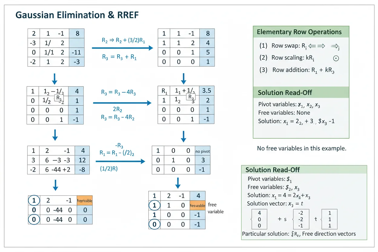
Reduced row echelon form is a standardized form of a matrix in which every nonzero row has a leading 1, every leading 1 is the only nonzero entry in its column, and successive pivots move to the right as you move down the matrix. It is often abbreviated RREF. A matrix is converted to reduced row echelon form using elementary row operations: swapping rows, multiplying a row by a nonzero scalar, and adding a multiple of one row to another. Unlike ordinary row echelon form, RREF eliminates entries both below and above every pivot. This makes solutions of linear systems, pivot variables, free variables, matrix rank, and consistency especially easy to identify. Every matrix has exactly one reduced row echelon form, even though many different sequences of row operations can produce it. RREF is therefore both a computational tool and a canonical representation of a matrix’s row-equivalence structure.
What Is Reduced Row Echelon Form?
A matrix is in reduced row echelon form when it satisfies all of the defining pivot conditions.
A typical RREF matrix looks like:
[ 1 0 a 0 b ]
[ 0 1 c 0 d ]
[ 0 0 0 1 e ]
[ 0 0 0 0 0 ]
The leading 1s are pivots.
In this example, the pivot columns are:
columns 1, 2, and 4
while columns 3 and 5 are nonpivot columns.
The number of pivots is:
3
so the matrix has rank 3.
Reduced Row Echelon Form Rules
A matrix is in reduced row echelon form if all of the following conditions hold.
Every row containing only zeros appears below all nonzero rows.
The first nonzero entry in each nonzero row is 1. This entry is called a leading 1 or pivot.
Each pivot lies strictly to the right of the pivot in the row above it.
Every pivot is the only nonzero entry in its entire column.
The last condition distinguishes reduced row echelon form from ordinary row echelon form.
Example of a Matrix in RREF
Consider:
[ 1 0 3 ]
[ 0 1 −2 ]
[ 0 0 0 ]
This matrix is in reduced row echelon form.
The first pivot is in column 1.
The second pivot is in column 2.
Both pivots equal 1, and each is the only nonzero value in its column.
The zero row appears at the bottom.
Column 3 is a nonpivot column.
Example That Is Not in RREF
Consider:
[ 1 2 0 ]
[ 0 1 3 ]
[ 0 0 0 ]
This matrix is in row echelon form, but it is not reduced.
The pivot in row 2 is:
1
but there is a:
2
above it in the same column.
For RREF, that entry must also be eliminated.
Perform:
R₁ → R₁ − 2R₂
to obtain:
[ 1 0 −6 ]
[ 0 1 3 ]
[ 0 0 0 ]
Now the matrix is in reduced row echelon form.
Elementary Row Operations
Only three elementary operations are needed to obtain RREF.
A row swap exchanges two rows:
Rᵢ ↔ Rⱼ
A row can be multiplied by any nonzero scalar c:
Rᵢ → cRᵢ
A multiple of one row can be added to another:
Rᵢ → Rᵢ + cRⱼ
These operations form the basis of row reduction.
They preserve the solution set of an augmented linear system when applied to the entire row, including the augmented column.
Why Row Operations Work
An augmented matrix represents a system of equations.
For example:
[ 1 1 | 5 ]
[ 2 −1 | 1 ]
represents:
x + y = 5
2x − y = 1
If one equation is replaced by itself plus a multiple of another equation, the system remains equivalent.
Likewise, changing equation order does not alter the solution set, and multiplying an equation by a nonzero constant produces an equivalent equation.
Matrix row operations encode these valid algebraic transformations compactly.
RREF Example: Solving a 3×3 System
Solve:
x + y + z = 6
2x − y + z = 3
x + 2y − z = 2
The augmented matrix is:
[ 1 1 1 | 6 ]
[ 2 −1 1 | 3 ]
[ 1 2 −1 | 2 ]
Use:
R₂ → R₂ − 2R₁
giving:
[ 1 1 1 | 6 ]
[ 0 −3 −1 | −9 ]
[ 1 2 −1 | 2 ]
Now:
R₃ → R₃ − R₁
so:
[ 1 1 1 | 6 ]
[ 0 −3 −1 | −9 ]
[ 0 1 −2 | −4 ]
Swap rows 2 and 3:
R₂ ↔ R₃
to obtain:
[ 1 1 1 | 6 ]
[ 0 1 −2 | −4 ]
[ 0 −3 −1 | −9 ]
Continue the Reduction
Eliminate the entry beneath the second pivot:
R₃ → R₃ + 3R₂
Then:
[ 1 1 1 | 6 ]
[ 0 1 −2 | −4 ]
[ 0 0 −7 | −21 ]
Scale row 3:
R₃ → −(1/7)R₃
giving:
[ 1 1 1 | 6 ]
[ 0 1 −2 | −4 ]
[ 0 0 1 | 3 ]
Now eliminate above the third pivot.
Use:
R₂ → R₂ + 2R₃
giving:
[ 1 1 1 | 6 ]
[ 0 1 0 | 2 ]
[ 0 0 1 | 3 ]
Then:
R₁ → R₁ − R₃
giving:
[ 1 1 0 | 3 ]
[ 0 1 0 | 2 ]
[ 0 0 1 | 3 ]
Finally:
R₁ → R₁ − R₂
The reduced row echelon form is:
[ 1 0 0 | 1 ]
[ 0 1 0 | 2 ]
[ 0 0 1 | 3 ]
Therefore:
x = 1
y = 2
z = 3
Why the Final Matrix Is Useful
The original system required three equations to be interpreted simultaneously.
The RREF matrix directly states:
x = 1
y = 2
z = 3
No back-substitution is necessary.
This is one advantage of reducing all the way to RREF rather than stopping at an upper-triangular echelon form.
RREF Versus Row Echelon Form
Row echelon form requires zeros below each pivot.
Reduced row echelon form requires zeros both below and above each pivot.
For example:
[ 1 2 3 ]
[ 0 1 4 ]
[ 0 0 1 ]
is in row echelon form but not RREF.
By eliminating upward:
[ 1 0 0 ]
[ 0 1 0 ]
[ 0 0 1 ]
can be obtained in this particular case.
Row echelon form is sufficient for back-substitution, whereas reduced form displays solutions and variable structure more directly.
Gauss–Jordan Elimination
The systematic procedure that continues elimination above as well as below every pivot is commonly called Gauss–Jordan elimination.
The broader RREF: Gauss–Jordan Elimination treatment focuses on that algorithmic viewpoint.
The reduced row echelon form itself is the canonical matrix produced at the end of the process.
Thus:
Gauss–Jordan elimination = procedure
while:
RREF = resulting canonical form
Uniqueness of RREF
A crucial fact is that every matrix has exactly one reduced row echelon form.
Different row-operation sequences may look very different.
For example, one solver may scale a pivot immediately, while another may eliminate several entries first.
If both calculations are correct and continued to full RREF, the final matrix must be identical.
This uniqueness makes RREF useful for checking independently performed reductions.
Pivot Columns
A pivot column contains a leading 1 in the RREF.
Consider:
[ 1 0 3 0 ]
[ 0 1 −2 0 ]
[ 0 0 0 1 ]
The pivot columns are:
1, 2, and 4
Column 3 is a nonpivot column.
The pivot positions reveal which variables are basic and which may be free in a linear system.
They also determine the matrix rank.
Matrix Rank From RREF
The rank equals the number of pivots:
rank(A) = number of pivot positions
For:
[ 1 0 2 3 ]
[ 0 1 −1 4 ]
[ 0 0 0 0 ]
there are two pivots.
Therefore:
rank(A) = 2
This remains the rank of the original matrix because elementary row operations preserve rank.
Free Variables
Suppose an augmented matrix reduces to:
[ 1 2 −1 | 3 ]
[ 0 0 0 | 0 ]
There is one pivot, in the x-column.
The variables y and z correspond to nonpivot columns and are free.
The equation is:
x + 2y − z = 3
Solve for x:
x = 3 − 2y + z
Let:
y = s
z = t
Then:
x = 3 − 2s + t
The system has infinitely many solutions because two free parameters remain.
Vector Form of an Infinite Solution Set
From:
x = 3 − 2s + t
y = s
z = t
write:
[x] [3] [−2] [1]
[y] = [0] + s [ 1] + t [0]
[z] [0] [ 0] [1]
This separates one particular solution from the independent null-space directions.
The number of free variables is closely related to rank and nullity.
Rank-Nullity Connection
If an m×n coefficient matrix A has n columns:
rank(A) + nullity(A) = n
The rank equals the number of pivot variables.
The nullity equals the number of free variables in:
Ax = 0
For example, if A has five columns and its RREF has three pivots:
rank(A) = 3
and:
nullity(A) = 5 − 3
= 2
So the homogeneous system has two independent free directions.
Unique Solution in RREF
For a system with n unknowns, a unique solution occurs when every variable column contains a pivot and the augmented system is consistent.
For three unknowns, a typical RREF is:
[ 1 0 0 | a ]
[ 0 1 0 | b ]
[ 0 0 1 | c ]
The solution is immediately:
x = a
y = b
z = c
There are no free variables.
No-Solution Example
Consider:
x + y = 2
2x + 2y = 5
The augmented matrix is:
[ 1 1 | 2 ]
[ 2 2 | 5 ]
Apply:
R₂ → R₂ − 2R₁
giving:
[ 1 1 | 2 ]
[ 0 0 | 1 ]
The second row represents:
0 = 1
which is impossible.
Therefore the system has no solution.
A contradiction row in RREF immediately exposes inconsistency.
Infinite-Solution Example
Consider:
x + 2y − z = 3
2x + 4y − 2z = 6
The second equation is twice the first.
Row reduction gives:
[ 1 2 −1 | 3 ]
[ 0 0 0 | 0 ]
There is only one independent equation for three unknowns.
Therefore two variables are free and the system has infinitely many solutions.
RREF and the Augmented Matrix
When solving:
Ax = b
form:
[A | b]
Row operations must be applied across the entire augmented row.
Changing only the coefficient entries without applying the same operation to the right-hand side changes the represented equations and invalidates the solution.
The augmented column is part of every row operation.
RREF and Matrix Inverses
Reduced row operations can be used to calculate a matrix inverse.
For a square matrix A, begin with:
[A | I]
and row-reduce.
If the left half becomes:
I
then the right half becomes:
A⁻¹
so:
[A | I] → [I | A⁻¹]
If the left side cannot be reduced to the identity, A is singular and has no ordinary inverse.
Small Inverse Example
Let:
A = [ 2 1 ]
[ 1 1 ]
Start with:
[ 2 1 | 1 0 ]
[ 1 1 | 0 1 ]
Reducing the left side to I produces:
[ 1 0 | 1 −1 ]
[ 0 1 | −1 2 ]
Therefore:
A⁻¹ = [ 1 −1 ]
[−1 2 ]
The result can be checked using matrix multiplication:
AA⁻¹ = I
RREF and the Determinant
For a square n×n matrix:
RREF(A) = I
if and only if A is invertible.
Equivalently:
det(A) ≠ 0
where det(A) is the matrix determinant.
If RREF contains a zero row before all n pivot columns are obtained, the matrix is rank deficient and:
det(A) = 0
RREF therefore reveals invertibility without directly computing the determinant.
RREF of an Invertible Matrix
For any invertible square matrix:
RREF(A) = I
For example:
A = [ 3 1 ]
[ 2 1 ]
has determinant:
3(1) − 1(2) = 1
Since the determinant is nonzero, A is invertible.
Its RREF must therefore be:
[ 1 0 ]
[ 0 1 ]
This is true regardless of the original entries.
RREF of a Singular Square Matrix
Consider:
A = [ 1 2 ]
[ 2 4 ]
Its rows are dependent.
Row reduction gives:
[ 1 2 ]
[ 0 0 ]
There is only one pivot.
Thus:
rank(A) = 1
and:
RREF(A) ≠ I
The matrix is singular.
RREF and Column Space
Pivot positions in RREF identify which columns of the original matrix form a basis for the column space.
Suppose the pivots occur in columns:
1, 3, and 5
Then select columns:
1, 3, and 5
from the original matrix.
Do not use the corresponding columns of the reduced matrix as a basis for the original column space, because row operations alter the actual column vectors.
This distinction is important when applying basis and dimension.
RREF and Row Space
The nonzero rows of an RREF matrix form a basis for the row space.
Unlike column-space basis extraction, the reduced rows themselves can be used directly.
For example:
[ 1 0 3 ]
[ 0 1 −2 ]
[ 0 0 0 ]
has row-space basis:
(1, 0, 3)
and:
(0, 1, −2)
The row space therefore has dimension:
2
which again equals the rank.
RREF and Null Space
RREF makes the equation:
Ax = 0
easy to solve.
Suppose:
RREF(A) = [ 1 0 2 ]
[ 0 1 −3 ]
Then:
x₁ + 2x₃ = 0
x₂ − 3x₃ = 0
Let:
x₃ = t
Then:
x₁ = −2t
x₂ = 3t
Therefore:
x = t(−2, 3, 1)
The null space has dimension 1.
RREF and Linear Transformations
For a linear transformation:
T(x) = Ax
RREF helps reveal the structural properties of A.
Pivot columns determine rank.
Free variables reveal null-space directions.
Full pivot structure can establish one-to-one or onto behavior when dimensions are appropriate.
However, row-reducing A changes the specific geometric transformation represented by the matrix, even though important linear-dependence information is preserved.
RREF should therefore be used to analyze structure rather than interpreted as the same geometric map.
RREF and Systems of Linear Equations
A system of linear equations is one of the main applications of RREF.
The final form can reveal:
one unique solution
infinitely many solutions
or:
no solution
without additional elimination.
The key visual signals are pivot columns, free-variable columns, and contradiction rows.
RREF and Matrix Operations
The broader matrix operations framework includes addition, multiplication, determinants, inverses, transposes, and row operations.
RREF specifically results from elementary row operations.
It is not obtained by performing ordinary matrix addition on entries or by simply dividing entire matrices.
Each row transformation must be one of the valid elementary operations.
RREF Is Not a Calculus Rule
Reduced row echelon form belongs to linear algebra and should not be confused with differentiation formulas such as the product rule, quotient rule, or power rule.
Those rules calculate derivatives of functions.
RREF instead transforms matrices while preserving row-equivalent linear-system information.
Likewise, related rates uses derivatives of quantities changing with time rather than matrix elimination.
The shared mathematical setting does not make these procedures interchangeable.
When to Stop at Row Echelon Form
If the only objective is solving a square system, ordinary echelon form followed by back-substitution may require fewer operations.
If the objective is to identify pivot variables, free variables, null spaces, rank, or a canonical row-equivalent matrix, continuing to RREF is usually more informative.
For an inverse calculation using:
[A | I]
full reduction to:
[I | A⁻¹]
is necessary.
The desired output determines how far the elimination should proceed.
Fractions During Reduction
Row reduction can create fractions.
They are mathematically harmless, but strategic choices can sometimes delay them.
For example, if a convenient pivot with value 1 is available in a lower row, swapping it upward may keep arithmetic simpler.
However, avoiding fractions at the expense of complicated row operations is not always worthwhile.
Accuracy matters more than keeping every intermediate entry integral.
RREF With Parameters
Some matrices contain parameters.
For example:
[ 1 a ]
[ 0 a−2 ]
The RREF depends on whether:
a − 2 = 0
If:
a ≠ 2
the second row contains a pivot after scaling.
If:
a = 2
the second row becomes zero and the rank drops.
Parameterized matrices therefore often require separate cases.
Common Reduced Row Echelon Form Mistakes
A common mistake is stopping when zeros exist only below pivots. That produces row echelon form, not necessarily reduced row echelon form.
Every pivot in RREF must equal 1.
Every pivot must also be the only nonzero entry in its column.
Zero rows must appear below nonzero rows.
When solving an augmented system, every row operation must include the augmented entry.
Dividing a row by zero is never permitted.
Another common error is treating a nonpivot variable as though it had a fixed numerical value; nonpivot variable columns generally indicate free parameters.
When finding a column-space basis, use the pivot columns from the original matrix rather than the reduced matrix.
Finally, different row-operation sequences may look different midway through the calculation, but a correctly completed RREF must be unique.
Frequently Asked Questions
What is reduced row echelon form?
Reduced row echelon form is a canonical matrix form in which every pivot is 1, every pivot is the only nonzero entry in its column, pivot positions move rightward down the matrix, and zero rows appear at the bottom.
What does RREF stand for?
RREF stands for reduced row echelon form.
What row operations can be used?
You may swap rows, multiply a row by a nonzero scalar, or add a multiple of one row to another.
What is the difference between REF and RREF?
Row echelon form requires zeros below pivots. Reduced row echelon form also requires zeros above pivots and makes every pivot equal to 1.
Is RREF unique?
Yes. Every matrix has exactly one reduced row echelon form.
How do you find matrix rank from RREF?
Count the pivot positions:
rank(A) = number of pivots
What does a free variable look like in RREF?
A variable corresponding to a nonpivot column is free.
How does RREF show a unique solution?
Every variable column has a pivot and there is no contradiction row.
How does RREF show infinitely many solutions?
The augmented system is consistent and at least one variable column has no pivot.
How does RREF show no solution?
A row such as:
[0 0 … 0 | 1]
represents an impossible equation and proves inconsistency.
How is RREF used to find an inverse?
Reduce:
[A | I]
to:
[I | A⁻¹]
If the left side cannot become I, A has no inverse.
Is RREF the same as Gauss–Jordan elimination?
RREF is the final matrix form. Gauss–Jordan elimination is the standard process used to reach it.
Can RREF identify a basis?
Yes. Pivot columns identify a basis for the original column space, while nonzero rows of RREF form a basis for the row space.
How can I check an RREF answer?
Confirm every pivot is 1, each pivot column contains zeros everywhere else, pivots move rightward down the rows, and all-zero rows are at the bottom.




