


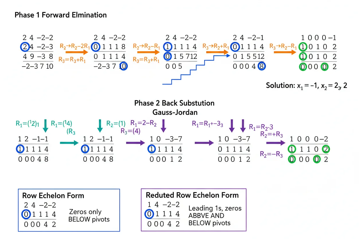
RREF, or reduced row echelon form, is the canonical matrix form produced by carrying Gauss–Jordan elimination through every pivot column. The method uses elementary row operations to create a leading 1 in each pivot position and zeros everywhere else in that pivot’s column. A fully reduced matrix places zero rows at the bottom, moves each successive pivot to the right, and leaves every pivot as the only nonzero entry in its column. This makes solutions to linear systems directly readable without back-substitution. Gauss–Jordan elimination can also expose free variables, detect inconsistent systems, calculate matrix rank, identify null-space parameters, and compute matrix inverses by reducing [A | I] to [I | A⁻¹]. The RREF of a matrix is unique even though many valid elimination sequences may lead to it. The practical challenge is therefore not choosing one mandatory sequence, but applying valid row operations accurately until every RREF condition is satisfied.
What Does RREF Mean?
RREF stands for:
Reduced Row Echelon Form
A typical RREF matrix is:
[ 1 0 3 0 ]
[ 0 1 −2 0 ]
[ 0 0 0 1 ]
[ 0 0 0 0 ]
The leading 1s are pivots.
Here they occur in columns:
1, 2, and 4
Each pivot is the only nonzero value in its column.
The zero row is at the bottom.
These structural conditions define the Reduced Row Echelon Form itself.
Gauss–Jordan elimination is the process used to reach it.
The Gauss–Jordan Elimination
Gauss–Jordan elimination extends ordinary elimination beyond row echelon form.
The general strategy is:
choose a pivot
make the pivot equal to 1
eliminate every other entry in the pivot column
move to the next pivot column
continue until all possible pivots are processed
At the end, the matrix is in RREF.
The broader row reduction framework contains both Gaussian and Gauss–Jordan elimination, while this process specifically continues until complete reduction.
The Three Permitted Row Operations
Gauss–Jordan elimination uses the same three elementary operations as any valid row-reduction procedure.
Swap two rows:
Rᵢ ↔ Rⱼ
Multiply a row by a nonzero constant:
Rᵢ → cRᵢ
where:
c ≠ 0
Add a multiple of one row to another:
Rᵢ → Rᵢ + cRⱼ
No other arbitrary entry changes are allowed.
Each operation must act on the full row.
RREF Conditions
A matrix is fully reduced only when all RREF requirements hold.
First, all zero rows appear below all nonzero rows.
Second, the first nonzero entry of every nonzero row is:
1
Third, each successive pivot appears farther right than the pivot above it.
Fourth, each pivot is the only nonzero entry in its column.
That final condition means eliminating entries both:
below the pivot
and:
above the pivot
This is what makes Gauss–Jordan elimination more extensive than ordinary forward Gaussian elimination.
REF Versus RREF
Consider:
[ 1 2 3 ]
[ 0 1 4 ]
[ 0 0 1 ]
This matrix is in row echelon form.
It is not in RREF because the second and third pivot columns contain nonzero entries above their pivots.
Continuing elimination can produce:
[ 1 0 0 ]
[ 0 1 0 ]
[ 0 0 1 ]
in this example.
Thus:
REF → zeros below pivots
while:
RREF → zeros above and below pivots
with every pivot normalized to 1.
Basic Gauss–Jordan Example
Solve:
x + y = 5
2x − y = 1
Construct:
[ 1 1 | 5 ]
[ 2 −1 | 1 ]
Eliminate beneath the first pivot:
R₂ → R₂ − 2R₁
giving:
[ 1 1 | 5 ]
[ 0 −3 | −9 ]
Normalize the second pivot:
R₂ → −(1/3)R₂
Then:
[ 1 1 | 5 ]
[ 0 1 | 3 ]
Finally eliminate above the second pivot:
R₁ → R₁ − R₂
The RREF is:
[ 1 0 | 2 ]
[ 0 1 | 3 ]
Therefore:
x = 2
y = 3
Why Gauss–Jordan Needs No Back-Substitution
Gaussian elimination could stop at:
[ 1 1 | 5 ]
[ 0 1 | 3 ]
and use:
y = 3
followed by:
x + 3 = 5
Gauss–Jordan continues until:
[ 1 0 | 2 ]
[ 0 1 | 3 ]
Now each equation contains only one pivot variable.
The solution can be read directly.
This is one of the defining practical advantages of RREF.
Three-Variable Gauss–Jordan Example
Solve:
x + y + z = 6
2x − y + z = 3
x + 2y − z = 2
Start with:
[ 1 1 1 | 6 ]
[ 2 −1 1 | 3 ]
[ 1 2 −1 | 2 ]
Eliminate entries below the first pivot:
R₂ → R₂ − 2R₁
R₃ → R₃ − R₁
giving:
[ 1 1 1 | 6 ]
[ 0 −3 −1 | −9 ]
[ 0 1 −2 | −4 ]
Swap:
R₂ ↔ R₃
to obtain a convenient pivot:
[ 1 1 1 | 6 ]
[ 0 1 −2 | −4 ]
[ 0 −3 −1 | −9 ]
Continue the Three-Variable Reduction
Eliminate beneath the second pivot:
R₃ → R₃ + 3R₂
Then:
[ 1 1 1 | 6 ]
[ 0 1 −2 | −4 ]
[ 0 0 −7 | −21 ]
Normalize the third pivot:
R₃ → −(1/7)R₃
giving:
[ 1 1 1 | 6 ]
[ 0 1 −2 | −4 ]
[ 0 0 1 | 3 ]
Now eliminate above the third pivot.
Use:
R₂ → R₂ + 2R₃
Then:
[ 1 1 1 | 6 ]
[ 0 1 0 | 2 ]
[ 0 0 1 | 3 ]
Next:
R₁ → R₁ − R₃
giving:
[ 1 1 0 | 3 ]
[ 0 1 0 | 2 ]
[ 0 0 1 | 3 ]
Finally:
R₁ → R₁ − R₂
The RREF is:
[ 1 0 0 | 1 ]
[ 0 1 0 | 2 ]
[ 0 0 1 | 3 ]
Therefore:
x = 1
y = 2
z = 3
RREF With a Free Variable
Consider:
[ 1 2 −1 | 3 ]
[ 2 4 −2 | 6 ]
Use:
R₂ → R₂ − 2R₁
giving:
[ 1 2 −1 | 3 ]
[ 0 0 0 | 0 ]
This matrix is already in RREF because the only pivot is:
1
in column 1 and it is the only nonzero entry in that column.
Variables y and z correspond to nonpivot columns.
Therefore they are free.
Let:
y = s
z = t
Then:
x + 2s − t = 3
so:
x = 3 − 2s + t
The system has infinitely many solutions.
Parametric Vector Form
The solution can be written:
[x] [3] [−2] [1]
[y] = [0] + s [ 1] + t [0]
[z] [0] [ 0] [1]
This representation separates:
one particular solution
from:
independent homogeneous directions
The number of free variables is the nullity of the coefficient matrix.
RREF With No Solution
Consider:
x + y = 2
2x + 2y = 5
The augmented matrix is:
[ 1 1 | 2 ]
[ 2 2 | 5 ]
Use:
R₂ → R₂ − 2R₁
Then:
[ 1 1 | 2 ]
[ 0 0 | 1 ]
The final row states:
0 = 1
which is impossible.
Therefore the system is inconsistent.
A contradiction row in RREF makes nonexistence of a solution immediately visible.
Unique, Infinite, or No Solutions
RREF makes the three main possibilities easy to distinguish.
A unique solution occurs when every variable is a pivot variable and no contradiction appears.
Infinitely many solutions occur when the system is consistent but at least one variable is free.
No solution occurs when a contradiction row appears.
This is why RREF is particularly useful for the complete structural analysis of linear systems.
Pivot Variables
A pivot variable corresponds to a pivot column in the coefficient part of an augmented matrix.
For:
[ 1 0 4 | 2 ]
[ 0 1 −3 | 5 ]
the x- and y-columns contain pivots.
So:
x and y
are pivot variables.
The z-column is nonpivot.
Therefore:
z
is free.
RREF and Matrix Rank
The matrix rank is the number of pivots in RREF.
For:
[ 1 0 2 0 ]
[ 0 1 −3 0 ]
[ 0 0 0 1 ]
there are:
3
pivots.
Therefore:
rank(A) = 3
Because RREF is unique, the pivot count is independent of which valid Gauss–Jordan sequence was chosen.
Full Rank and RREF
For an n×n square matrix:
rank(A) = n
if and only if:
RREF(A) = Iₙ
So a 3×3 matrix is full rank exactly when its RREF is:
[ 1 0 0 ]
[ 0 1 0 ]
[ 0 0 1 ]
Full rank is equivalent to invertibility for a square matrix.
RREF and Matrix Inverses
Gauss–Jordan elimination provides a direct way to calculate a matrix inverse.
Start with:
[A | I]
Apply row operations until the left side becomes I.
If successful:
[A | I] → [I | A⁻¹]
Every operation that turns A into I simultaneously builds the inverse on the right.
If A cannot reduce to I, it has no ordinary inverse.
Inverse Example With Gauss–Jordan
Let:
A = [ 2 1 ]
[ 1 1 ]
Begin:
[ 2 1 | 1 0 ]
[ 1 1 | 0 1 ]
Swap the rows:
[ 1 1 | 0 1 ]
[ 2 1 | 1 0 ]
Eliminate:
R₂ → R₂ − 2R₁
giving:
[ 1 1 | 0 1 ]
[ 0 −1 | 1 −2 ]
Normalize:
R₂ → −R₂
so:
[ 1 1 | 0 1 ]
[ 0 1 | −1 2 ]
Eliminate above:
R₁ → R₁ − R₂
Then:
[ 1 0 | 1 −1 ]
[ 0 1 | −1 2 ]
Therefore:
A⁻¹ = [ 1 −1 ]
[−1 2 ]
Why the Inverse Method Works
Every row operation can be represented by an elementary matrix.
Suppose the sequence of operations is:
Eₖ…E₂E₁
and:
Eₖ…E₂E₁A = I
Multiply by A⁻¹ conceptually:
Eₖ…E₂E₁ = A⁻¹
When the same operations are applied to I, they produce exactly this product of elementary matrices.
That is why the right half of:
[A | I]
becomes A⁻¹ when the left half becomes I.
RREF and the Determinant
For a square matrix:
RREF(A) = I
if and only if:
det(A) ≠ 0
where the determinant is the matrix determinant.
If the matrix is singular, Gauss–Jordan elimination eventually reveals fewer than n pivots.
The RREF then cannot be the identity matrix.
Thus RREF provides an invertibility test without explicitly computing the determinant.
RREF and Matrix Multiplication
The elementary operations underlying Gauss–Jordan elimination can be represented through matrix multiplication.
A row swap, row scaling, or row replacement corresponds to left multiplication by an elementary matrix.
Therefore a complete reduction can be represented:
Eₖ…E₂E₁A = R
where R is the RREF of A.
This provides an algebraic interpretation of the elimination algorithm.
RREF and Matrix Operations
Gauss–Jordan elimination is one part of the wider matrix operations framework.
It should not be confused with ordinary matrix addition or standard matrix multiplication.
The entries are changed only through complete row operations.
Those operations preserve row equivalence while revealing structural information such as rank, nullity, and linear-system consistency.
RREF and Basis
Suppose the pivot columns of RREF occur in positions:
1, 3, and 5
Then columns 1, 3, and 5 of the original matrix identify a basis for its column space.
The actual original columns must be used because row operations change column vectors.
The number of these pivot columns equals the dimension of the column space, tying RREF directly to basis and dimension.
Basis for the Row Space
The nonzero rows of RREF form a basis for the row space.
For example:
[ 1 0 2 3 ]
[ 0 1 −1 4 ]
[ 0 0 0 0 ]
has row-space basis:
(1, 0, 2, 3)
and:
(0, 1, −1, 4)
The row-space dimension is therefore:
2
which agrees with the matrix rank.
RREF and the Null Space
RREF is especially convenient for solving:
Ax = 0
Suppose:
RREF(A) = [ 1 0 2 ]
[ 0 1 −3 ]
The equations are:
x₁ + 2x₃ = 0
x₂ − 3x₃ = 0
Let:
x₃ = t
Then:
x₁ = −2t
x₂ = 3t
Therefore:
x = t(−2, 3, 1)
The null space is one-dimensional.
Rank-Nullity From RREF
If A has n columns:
rank(A) + nullity(A) = n
RREF exposes both quantities immediately.
The number of pivots is the rank.
The number of nonpivot variable columns is the nullity.
For a matrix with:
6 columns
and:
4 pivots
we have:
rank = 4
nullity = 2
RREF and Linear Transformations
For a linear transformation:
T(x) = Ax
RREF can reveal whether the transformation has a nontrivial kernel, whether its columns span the codomain, and how many independent output directions exist.
However, RREF(A) is generally not the same geometric transformation as A.
Row operations preserve algebraic solution relationships, not the full geometric action of the original matrix.
One-to-One Behavior
For a transformation represented by an m×n matrix A, the map is one-to-one when:
Ax = 0
has only the trivial solution.
In RREF language, this requires a pivot in every variable column.
Therefore:
no free variables → trivial kernel → one-to-one
when interpreted for the corresponding matrix transformation.
Onto Behavior
A transformation:
T: Rⁿ → Rᵐ
is onto Rᵐ when the column space has dimension m.
In RREF terms, this requires a pivot in every row of the coefficient matrix.
Thus RREF reveals both one-to-one and onto structure through pivot placement.
For a square matrix, having a pivot in every row and every column are equivalent and imply invertibility.
RREF and Systems of Linear Equations
For:
Ax = b
Gauss–Jordan elimination transforms:
[A | b]
into a form from which every variable relationship can be read directly.
The algorithm simultaneously answers:
Is the system consistent?
Which variables are pivots?
Which variables are free?
Is the solution unique?
What is the rank?
This is why RREF is more informative than merely obtaining one numerical solution.
RREF With More Equations Than Unknowns
Consider a system with:
4 equations
and:
2 unknowns
Its augmented matrix has four rows but only two coefficient columns.
Gauss–Jordan elimination may reveal redundant equations as zero rows.
If both variable columns contain pivots and no contradiction occurs, the system can still have a unique solution.
Having more equations than variables does not automatically imply inconsistency.
The independence of the equations matters.
RREF With More Unknowns Than Equations
If a consistent system has:
2 equations
and:
4 unknowns
there can be at most two pivot variables.
At least two variables must therefore remain free.
The system cannot have a unique solution.
RREF makes this dimensional limitation immediately visible.
Choosing Convenient Pivots
Suppose the leading column is:
[ 4 ]
[ 1 ]
[−2 ]
All three entries are nonzero, but swapping the row containing:
1
to the top may keep subsequent arithmetic simpler.
Gauss–Jordan elimination permits such a swap.
A convenient pivot can reduce fractions and arithmetic errors without affecting the final RREF.
Fractions in Gauss–Jordan Elimination
Fractions are sometimes unavoidable.
For example, a pivot:
7
must eventually be normalized to:
1
by multiplying the row by:
1/7
It is valid to postpone that scaling if elimination remains easier with integer arithmetic.
What matters is that every pivot equals 1 in the final RREF.
Intermediate matrices do not need to satisfy the final normalization conditions.
RREF With Parameters
Consider:
A = [ 1 2 ]
[ 0 a−4 ]
If:
a ≠ 4
then the second row can be scaled to produce a second pivot.
Thus:
RREF(A) = I
after appropriate elimination.
If:
a = 4
the second row becomes zero, so only one pivot remains.
Parameterized Gauss–Jordan problems therefore require separate cases when a potential pivot can vanish.
Numerical Stability
For hand calculations using exact numbers, any nonzero pivot is mathematically valid.
In floating-point computation, dividing by an extremely small pivot can magnify numerical error.
Practical numerical elimination algorithms often swap rows to use a larger pivot.
This does not change the theoretical RREF concept, although floating-point implementations may return values that are only numerically close to exact zeros and ones.
RREF and the Identity Matrix
For every invertible square matrix A:
RREF(A) = I
This provides a concise characterization of invertibility.
If A is 4×4 and Gauss–Jordan elimination yields four pivots, the final reduced matrix is:
I₄
If fewer than four pivots remain, A is singular.
RREF Is Unique
The RREF of every matrix is unique.
Suppose two students begin with the same matrix but choose different valid row swaps and replacement operations.
Their intermediate matrices can differ.
If both calculations are correct and both continue until true RREF is reached, their final matrices must match exactly.
This provides a strong verification property.
Intermediate Matrices Are Not Unique
Uniqueness applies only to the final reduced row echelon form.
There are usually many possible elimination paths.
For example, one method may:
scale a pivot first
while another may:
use the unscaled pivot to eliminate entries first
Both are valid.
The important requirement is that every operation is elementary and applied consistently.
Gauss–Jordan Versus Gaussian Elimination
Gaussian elimination focuses on forward elimination.
It creates an echelon form such as:
[ 1 a b ]
[ 0 1 c ]
[ 0 0 1 ]
and then uses back-substitution.
Gauss–Jordan continues upward elimination:
[ 1 0 0 ]
[ 0 1 0 ]
[ 0 0 1 ]
when the square system is full rank.
Gauss–Jordan usually requires more arithmetic but leaves the solution directly visible.
When RREF Is Especially Useful
Full RREF is particularly useful when the problem asks for more than one solution value.
Examples include determining:
free variables
parametric solution sets
matrix rank
null-space bases
column-space pivot positions
inverse matrices
consistency conditions
When only one numerical solution to a large system is needed, stopping at echelon form and back-substituting may be computationally cheaper.
RREF Versus Calculus Procedures
RREF is specifically a linear algebra elimination method. It should not be confused with calculus procedures simply because they may also involve several equations.
A Separable Differential Equation is handled by separating variables and integrating. Related Rates differentiates quantities that change with time. A Surface Area Of Revolution problem evaluates a geometric integral.
Gauss–Jordan elimination instead applies elementary operations to matrix rows.
Choosing the method depends on the mathematical structure of the problem, not merely on the number of variables present.
RREF and the Broader Calculus & Linear Algebra Framework
Within Calculus & Linear Algebra, RREF is fundamentally a linear algebra tool.
Its main role is to reveal the structure encoded by a matrix.
It connects directly with:
- linear systems,
- matrix rank,
- inverses,
- bases,
- null spaces,
- and linear transformations.
Its value comes from making hidden dependence and solution structure explicit.
Checking a Gauss–Jordan Calculation
First verify every row step individually.
For a row replacement such as:
R₃ → R₃ − 2R₁
recalculate every entry in row 3, including any augmented entries.
At the end, inspect the matrix structurally.
Every nonzero row must have a leading 1.
Each pivot must be the only nonzero value in its column.
Pivot positions must move right as you move down.
Zero rows must be at the bottom.
If the original problem is a linear system, substitute the resulting solution into the original equations for an additional check.
Common RREF Mistakes
A common mistake is stopping at ordinary row echelon form and calling it RREF.
Another is failing to normalize a pivot to 1.
Entries above pivots must be eliminated as well as those below.
Every operation must apply to the entire row, including the augmented column.
Multiplying a row by zero is invalid.
When free variables exist, they should be assigned parameters rather than arbitrarily set to zero unless one particular solution is specifically desired.
For a column-space basis, use pivot columns from the original matrix rather than from RREF.
Students may also expect identical intermediate steps from different solutions. Only the final RREF is unique.
Finally, Gauss–Jordan elimination should not be continued mechanically without checking arithmetic after each major pivot. One small sign error can affect every later row.
Frequently Asked Questions
What does RREF stand for?
RREF stands for reduced row echelon form.
What is Gauss–Jordan elimination?
Gauss–Jordan elimination is the row-operation process that reduces a matrix all the way to RREF.
What are the three allowed Gauss–Jordan row operations?
You may swap two rows, multiply a row by a nonzero scalar, or add a multiple of one row to another.
What makes RREF different from row echelon form?
RREF requires every pivot to equal 1 and to be the only nonzero entry in its column. Row echelon form requires zeros below pivots but not necessarily above them.
Is the RREF of a matrix unique?
Yes. Every matrix has exactly one RREF.
Are the Gauss–Jordan steps unique?
No. Many valid row-operation sequences can lead to the same final RREF.
How do you identify matrix rank from RREF?
Count the pivots:
rank(A) = number of pivots
How does RREF show a free variable?
Any variable column without a pivot corresponds to a free variable.
How does RREF show no solution?
A contradiction row such as:
[0 0 … 0 | 1]
shows that the system is inconsistent.
How does RREF show infinitely many solutions?
The system is consistent and at least one variable column lacks a pivot.
How do you find an inverse using Gauss–Jordan elimination?
Reduce:
[A | I]
to:
[I | A⁻¹]
If the left side cannot become I, A is not invertible.
What is RREF for an invertible square matrix?
It is the identity matrix:
RREF(A) = I
Is Gauss–Jordan elimination the same as Gaussian elimination?
No. Gaussian elimination generally stops at echelon form and uses back-substitution. Gauss–Jordan continues until full RREF.
How can I verify an RREF result?
Check the pivot conditions, verify each recorded row operation, and confirm any resulting linear-system solution in the original equations.




