


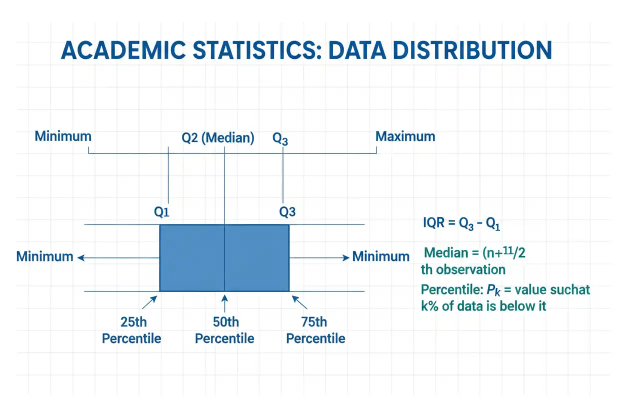
Quartiles are measures of position that divide an ordered data set or probability distribution into four broad sections, making them especially useful for describing center, spread, skewness, and the location of observations without relying heavily on extreme values. The three principal quartiles are Q₁, which corresponds conceptually to the 25th percentile; Q₂, which is the median or 50th percentile; and Q₃, which corresponds conceptually to the 75th percentile. Together, they identify the boundaries around the middle half of a distribution, and the distance Q₃ − Q₁ defines the interquartile range, a robust measure of dispersion that is widely used in box plots and outlier screening. Unlike the arithmetic mean, quartiles depend primarily on ordered position rather than the precise magnitude of every observation, so a very large or very small extreme value may have little effect on the central quartiles. However, there is no single universally adopted finite-sample formula for calculating Q₁ and Q₃, which means different textbooks, calculators, and software systems can return slightly different quartiles for the same small sample. Correct interpretation therefore requires both understanding what quartiles represent and recognizing which ranking or interpolation convention was used to calculate them.
Quartiles belong to the descriptive tools within core statistics and the broader Statistics & Probability framework. Their meaning is grounded in cumulative probability, while their stability and precision depend partly on sample size because small samples provide relatively little information about specific distributional positions.
What Are Quartiles?
Quartiles divide ordered observations into four sections associated with cumulative positions of approximately:
25%
50%
75%
The three quartile values are conventionally written:
Q₁ = first quartile
Q₂ = second quartile
Q₃ = third quartile
Conceptually:
Q₁ ≈ 25th percentile
Q₂ = 50th percentile = median
Q₃ ≈ 75th percentile
The word “approximately” matters for finite samples because different quantile conventions define the exact sample positions differently. At the population-distribution level, quartiles are naturally tied to cumulative probabilities of 0.25, 0.50, and 0.75.
What Does Q₁ Mean?
The first quartile, Q₁, marks the lower-quarter boundary of an ordered distribution. In a continuous population distribution, Q₁ is a value associated with cumulative probability:
P(X ≤ Q₁) = 0.25
under the usual quantile interpretation.
In sample data, Q₁ is calculated from ordered observations using a specified quartile convention. A common informal interpretation is that roughly:
25%
of observations lie at or below Q₁ and roughly:
75%
lie at or above it.
Ties and interpolation can make those percentages imperfect in finite samples, so Q₁ should be understood primarily as the lower quartile position rather than as a guarantee of an exact 25/75 split in every data set.
What Does Q₂ Mean?
The second quartile is the median:
Q₂ = Median
It divides an ordered distribution into lower and upper halves.
For an odd number of observations, Q₂ is usually the middle ordered value.
For an even number of observations, the conventional sample median is generally the average of the two middle values.
Because Q₂ is the median, it is resistant to isolated extreme magnitudes in the same way the median is.
What Does Q₃ Mean?
The third quartile, Q₃, marks the upper-quarter boundary.
At the population level, it corresponds conceptually to:
P(X ≤ Q₃) = 0.75
for a suitable continuous distribution.
In sample data, Q₃ locates the upper portion of the central half of observations.
Approximately:
75%
of observations lie at or below Q₃
and:
25%
lie above it,
subject again to the calculation convention, ties, and discreteness of the data.
Quartiles Formula
There is no single universal finite-sample quartiles formula, but several widely used methods exist.
One common approach is to find:
Q₂ = median of the full ordered data
then calculate:
Q₁ = median of the lower half
and:
Q₃ = median of the upper half.
This is often called a median-of-halves approach.
Another widely used method treats quartiles as interpolated sample quantiles. A common position formula is:
h = 1 + (n − 1)q
where:
- n = number of observations
- q = target cumulative proportion
For:
Q₁, q = 0.25
For:
Q₂, q = 0.50
For:
Q₃, q = 0.75
When h lies between two integer positions, the quartile is linearly interpolated between the corresponding ordered observations.
Why Quartile Formulas Differ
A finite sample contains only n observed positions, while quartiles conceptually represent exact 25%, 50%, and 75% cumulative locations. When those conceptual positions fall between observed data points, a calculation method must decide whether to select one observation, average observations, include or exclude the overall median when splitting the sample, or interpolate between neighboring values.
That choice creates different legitimate finite-sample conventions. For large data sets, the numerical differences are often small relative to the distribution’s scale, but in small samples they can be noticeable. Consequently, a quartile calculation is not fully reproducible unless the convention or software definition is known.
How to Calculate Quartiles
A practical quartile calculation begins by sorting all observations from smallest to largest. The calculation method is then applied consistently to the ordered sequence, with Q₂ determined as the median and Q₁ and Q₃ determined from the selected lower- and upper-distribution positions.
Consider the ordered data:
2, 4, 5, 7, 8, 10, 12, 15, 18, 21
There are:
n = 10
observations.
Using the median-of-halves convention, the two middle values are:
8 and 10
Therefore:
Q₂ = (8 + 10)/2
Q₂ = 9
The lower half is:
2, 4, 5, 7, 8
Its median is:
5
so:
Q₁ = 5
The upper half is:
10, 12, 15, 18, 21
Its median is:
15
so:
Q₃ = 15
Therefore:
Q₁ = 5
Q₂ = 9
Q₃ = 15
under this convention.
Quartiles Example With Odd Sample Size
Consider:
2, 4, 6, 7, 9, 11, 13, 15, 20
There are:
n = 9
observations.
The middle observation is the fifth:
Q₂ = 9
One common median-of-halves convention excludes the overall median when calculating Q₁ and Q₃.
The lower half becomes:
2, 4, 6, 7
Therefore:
Q₁ = (4 + 6)/2
Q₁ = 5
The upper half becomes:
11, 13, 15, 20
Therefore:
Q₃ = (13 + 15)/2
Q₃ = 14
The quartile summary is:
Q₁ = 5
Q₂ = 9
Q₃ = 14
Another convention may include the overall median in each half and therefore produce different Q₁ and Q₃ values. That difference comes from methodology rather than necessarily from arithmetic error.
Interpolated Quartiles
Return to:
2, 4, 5, 7, 8, 10, 12, 15, 18, 21
Using:
h = 1 + (n − 1)q
with:
n = 10
for Q₁:
h = 1 + 9(0.25)
h = 3.25
The target lies 25% of the way from the third observation to the fourth.
Those values are:
5 and 7
Therefore:
Q₁ = 5 + 0.25(7 − 5)
Q₁ = 5.5
For Q₃:
h = 1 + 9(0.75)
h = 7.75
The seventh and eighth observations are:
12 and 15
Therefore:
Q₃ = 12 + 0.75(15 − 12)
Q₃ = 14.25
Under this interpolation convention:
Q₁ = 5.5
Q₂ = 9
Q₃ = 14.25
The median-of-halves method produced:
Q₁ = 5
Q₃ = 15
Both results can be legitimate when their conventions are stated clearly.
Quartiles and Percentiles
Quartiles are special percentile positions.
The conceptual relationships are:
Q₁ = P25
Q₂ = P50
Q₃ = P75
Therefore, quartiles divide a distribution into four broad probability sections, while percentiles divide it conceptually into one hundred positions.
The same underlying idea is involved: ordered cumulative position.
Quartiles provide a compact summary, whereas a fuller percentile profile can describe more detailed tail behavior.
Quartiles and Deciles
Deciles divide an ordered distribution into ten sections.
Examples include:
D₁ = 10th percentile
D₅ = 50th percentile
D₉ = 90th percentile
Therefore:
Q₂ = D₅ = P50
All of these measures belong to the general family of quantiles.
Their differences are primarily the granularity with which they divide cumulative probability.
Interquartile Range
The interquartile range is:
IQR = Q₃ − Q₁
It measures the width of the middle 50% of a distribution.
Using the median-of-halves result:
Q₁ = 5
Q₃ = 15
we obtain:
IQR = 15 − 5
IQR = 10
Unlike the overall range, the IQR does not depend directly on the minimum and maximum observations. It is therefore much less sensitive to isolated extreme values.
Why the IQR Is Robust
Suppose the data are:
2, 4, 5, 7, 8, 10, 12, 15, 18, 21
and Q₁ and Q₃ under a chosen method are determined by values well inside the sample.
Now replace:
21
with:
2,100
The maximum changes dramatically, and the arithmetic mean will also increase substantially.
However, the central quartile positions may remain unchanged because the extreme value still occupies the highest rank.
This resistance makes quartiles and the IQR useful when data are skewed or contain legitimate extreme observations.
Quartiles vs Range
The ordinary range is:
Range = Maximum − Minimum
For:
2, 4, 5, 7, 8, 10, 12, 15, 18, 21
the range is:
21 − 2
= 19
If the maximum changes from:
21
to:
2,100
the range becomes:
2,098
even though nine of the ten observations remain unchanged.
The IQR, by contrast, can stay roughly the same because it focuses on the central half of the data.
The range describes total span. The IQR describes central spread.
Quartiles and the Five-Number Summary
Quartiles are central components of the five-number summary:
Minimum
Q₁
Median
Q₃
Maximum
For example:
Minimum = 2
Q₁ = 5
Median = 9
Q₃ = 15
Maximum = 21
This compact summary provides information about location, spread, and potential asymmetry.
The distances between consecutive values can reveal whether one side of the distribution extends farther than the other.
Quartiles and Box Plots
A box plot visualizes quartile structure.
The box commonly extends from:
Q₁ to Q₃
with a line at:
Q₂
or the median.
Therefore, the width or length of the box represents:
IQR = Q₃ − Q₁
Whiskers extend outward according to the box-plot convention being used, often toward observations that remain within calculated 1.5×IQR fences.
Observations beyond the whiskers may then be displayed individually as potential outliers.
The quartiles form the central architecture of the box plot.
Quartiles and Outlier Fences
A common exploratory rule uses:
Lower fence = Q₁ − 1.5(IQR)
and:
Upper fence = Q₃ + 1.5(IQR)
Suppose:
Q₁ = 5
Q₃ = 15
Then:
IQR = 10
The fences are:
Lower = 5 − 15
= −10
and:
Upper = 15 + 15
= 30
An observation above 30 or below −10 would be flagged under this rule.
The quartiles determine the central reference points, while the IQR determines how far the screening boundaries extend.
A Flagged Observation Is Not Automatically an Error
The 1.5×IQR rule is a descriptive screening method.
If an observation lies beyond a quartile-based fence, that means it is unusually far from the central quartile range under the selected rule. It does not establish that the value was recorded incorrectly or that it belongs to another population.
A flagged observation can represent a legitimate tail event, measurement error, a new subgroup, a structural change, or an unsuitable probability model. Statistical investigation should therefore follow the flag rather than automatic deletion.
Quartiles and the Median
The median is:
Q₂
so quartile analysis automatically contains one of the most important measures of central tendency.
Suppose:
Q₁ = 20
Q₂ = 25
Q₃ = 50
The median lies much closer to Q₁ than Q₃.
That pattern can indicate greater spread within the upper half of the central 50% than within the lower half.
However, quartile spacing alone cannot completely describe distribution shape.
Histograms, density plots, and additional percentiles can provide further information.
Quartiles and Skewness
Quartile spacing can provide descriptive clues about asymmetry.
Suppose:
Q₁ = 10
Q₂ = 20
Q₃ = 60
The distance above the median is:
Q₃ − Q₂ = 40
while the distance below is:
Q₂ − Q₁ = 10
The central distribution extends much farther upward than downward.
This is consistent with right-skewed behavior within the middle portion of the data.
However, skewness concerns the entire distribution, including tails, so quartile spacing should be treated as evidence rather than a universal diagnostic rule.
Bowley’s Quartile Skewness
A quartile-based skewness measure sometimes called Bowley’s coefficient is:
Skewness_Q = (Q₃ + Q₁ − 2Q₂)/(Q₃ − Q₁)
provided:
Q₃ ≠ Q₁
An equivalent form is:
Skewness_Q = [(Q₃ − Q₂) − (Q₂ − Q₁)]/(Q₃ − Q₁)
If the quartile spacing is symmetric around the median:
Q₃ − Q₂ = Q₂ − Q₁
then:
Skewness_Q = 0
Positive values indicate relatively greater upper-half spread, while negative values indicate greater lower-half spread.
Because the measure uses quartiles, it is comparatively resistant to extreme tail magnitudes.
Quartile Skewness Example
Suppose:
Q₁ = 10
Q₂ = 20
Q₃ = 50
Then:
Skewness_Q = (50 + 10 − 40)/(50 − 10)
= 20/40
= 0.5
This positive value reflects greater spacing above the median.
The calculation should not be interpreted as equivalent to moment-based skewness. The measures use different information and can produce different numerical values.
Quartile skewness is specifically a robust positional description.
Quartile Coefficient of Dispersion
Another quartile-based measure sometimes used for positive-valued data is:
Coefficient = (Q₃ − Q₁)/(Q₃ + Q₁)
provided the denominator is meaningful and nonzero.
For:
Q₁ = 20
Q₃ = 30
we obtain:
(30 − 20)/(30 + 20)
= 10/50
= 0.20
This measure expresses central quartile spread relative to the quartile magnitudes.
Its usefulness depends on the measurement scale and analytical context.
Quartiles in Symmetric Data
For a symmetric population distribution centered at m, Q₁ and Q₃ are equally spaced around the center:
m − Q₁ = Q₃ − m
when the quartiles are uniquely defined in the usual way.
Thus:
Q₁ + Q₃ = 2m
For a symmetric distribution whose mean and median coincide at μ:
Q₁ = μ − d
Q₃ = μ + d
for some positive d.
This symmetry is especially useful in the normal distribution.
Quartiles of the Normal Distribution
For:
X ~ N(μ, σ²)
the standard normal 25th percentile is approximately:
z₀.₂₅ ≈ −0.67449
and the 75th percentile is:
z₀.₇₅ ≈ 0.67449
Therefore:
Q₁ ≈ μ − 0.67449σ
Q₂ = μ
Q₃ ≈ μ + 0.67449σ
The normal-distribution IQR is therefore:
IQR ≈ 1.34898σ
or approximately:
IQR ≈ 1.349σ
This relationship is specific to a normal population and should not be used as a universal conversion between IQR and standard deviation.
Converting Normal IQR to Standard Deviation
Under an exact normal model:
IQR ≈ 1.349σ
Therefore:
σ ≈ IQR/1.349
For example, if a normal population has:
IQR = 13.49
then:
σ ≈ 13.49/1.349
σ ≈ 10
This conversion can be useful when robust central-spread summaries are available but the model is assumed normal.
Without the normal-distribution assumption, the relationship need not hold.
Quartiles in Uniform Data
For a continuous uniform distribution on:
[a,b]
the cumulative distribution increases linearly.
Therefore:
Q₁ = a + 0.25(b − a)
Q₂ = a + 0.50(b − a)
Q₃ = a + 0.75(b − a)
The quartiles are equally spaced.
For a uniform distribution on:
[0,100]
we have:
Q₁ = 25
Q₂ = 50
Q₃ = 75
This provides a simple example where quartile positions correspond directly to equal numerical intervals.
Quartiles in Skewed Distributions
In a skewed distribution, quartiles need not be equally spaced.
Suppose:
Q₁ = 5
Q₂ = 8
Q₃ = 20
Then the lower central-quarter distance is:
8 − 5 = 3
while the upper distance is:
20 − 8 = 12
This asymmetry indicates that the upper middle portion is much more spread out than the lower middle portion.
Because quartiles are resistant to extreme tail values, they can provide a useful summary of skewed distributions in which the arithmetic mean and standard deviation are strongly influenced by a few large observations.
Quartiles in Discrete Distributions
Discrete probability distributions have cumulative distribution functions that move in jumps.
Therefore, an exact cumulative probability of:
0.25
or:
0.75
may not occur at any possible count.
A common population quantile definition selects the smallest value x for which:
F(x) ≥ q
where q is the desired quantile level.
Consequently, several quartiles can sometimes have the same value, particularly when much probability mass is concentrated on a few integer outcomes.
This is not a calculation error; it reflects the discrete distribution.
Quartiles of a Poisson Distribution
The Poisson distribution provides a clear example of discrete quartiles.
If:
X ~ Poisson(λ)
the first quartile can be defined as the smallest integer k satisfying:
P(X ≤ k) ≥ 0.25
The median is the smallest k satisfying an appropriate 0.50 quantile definition, and Q₃ similarly uses:
P(X ≤ k) ≥ 0.75
Because the Poisson CDF jumps at integer counts, the cumulative probabilities at these selected values will often exceed exactly 25%, 50%, or 75%.
Repeated Values and Quartiles
Ties can produce identical quartiles.
Suppose:
0, 0, 0, 0, 0, 1, 1, 1, 1
Depending on the quartile convention:
Q₁ = 0
Q₂ = 0
while:
Q₃
may equal 1 or another boundary determined by the method.
A quartile does not need to identify a unique observation with precisely 25% of values below it.
In discrete or heavily tied data, cumulative probability can concentrate at the same numerical value across a range of quantile levels.
Zero Interquartile Range
If:
Q₁ = Q₃
then:
IQR = 0
This means the middle half of the distribution has no numerical spread under the selected quartile definition.
For example, a data set containing many repeated values can have:
Q₁ = Q₂ = Q₃ = 5
even though a few observations differ substantially from 5.
A zero IQR therefore does not necessarily mean that every observation is identical.
It means the central quartile range collapses to one value.
Quartiles and Small Samples
Quartiles can be unstable in small samples because relatively few observations determine the relevant positions.
Suppose:
n = 5
A change in a single observation can alter an entire quartile substantially.
Different finite-sample formulas can also generate visibly different results because the positions corresponding to 25% and 75% lie between a small number of observed ranks.
This is one reason sample size matters when interpreting quartile estimates from data.
A numerically precise Q₁ or Q₃ does not imply that the corresponding population quartile has been estimated with high precision.
Quartiles and Large Samples
As sample size grows, empirical quartiles can generally estimate population quartiles more precisely under suitable independent sampling conditions.
However, a large sample does not correct:
- systematic sampling bias,
- measurement error,
- changing populations,
- dependence ignored by the design.
A precisely estimated quartile from an unrepresentative sample can still be a poor estimate of the target population’s quartile.
Sample size addresses random sampling variability, not every source of error.
Sample Quartiles vs Population Quartiles
Sample quartiles are statistics calculated from observed data.
Population quartiles are fixed characteristics of a population distribution.
Different random samples from the same population can produce different:
Q₁
Q₂
Q₃
because the sample contains different observations.
For example, two samples might produce:
Sample A Q₁ = 20
and:
Sample B Q₁ = 23
even though both were drawn from a population whose true Q₁ is:
21.5
Sampling variability is therefore distinct from the methodological differences caused by alternative quartile formulas.
Quartiles and Weighted Data
Some observations can carry unequal statistical weights.
In that case, weighted quartiles are based on cumulative weight rather than simply cumulative observation count.
Suppose one record represents:
1 individual
and another represents:
500 individuals.
Treating them as equal can misrepresent the intended population distribution.
A weighted quartile procedure sorts observations and accumulates their weights until the target proportion of total weight is reached.
Exact interpolation conventions can still differ, so weighted quartile methodology should be documented when results are consequential.
Quartiles From Frequency Tables
Quartiles can also be obtained from discrete frequency tables.
Suppose:
| Value | Frequency |
|---|---|
| 1 | 2 |
| 2 | 4 |
| 3 | 6 |
| 4 | 5 |
| 5 | 3 |
The total number of observations is:
N = 20
Cumulative frequencies are:
Value 1 → 2
Value 2 → 6
Value 3 → 12
Value 4 → 17
Value 5 → 20
The 25% cumulative position is around:
5th observation
which lies at value:
2
The median lies around the:
10th and 11th observations
which both lie at value:
3
The 75% position is around:
15th observation
which lies at value:
4
Therefore, under a natural rank interpretation:
Q₁ = 2
Q₂ = 3
Q₃ = 4
Quartiles From Grouped Continuous Data
When only grouped intervals are available, exact quartiles usually cannot be recovered because the individual values inside each interval are unknown.
An interpolated grouped-data formula is often used:
Qq = L + [(qN − CF)/f]w
where:
- q = 0.25, 0.50, or 0.75
- L = lower boundary of the quartile class
- N = total frequency
- CF = cumulative frequency before the quartile class
- f = frequency within that class
- w = class width
This estimates where the quartile lies within the relevant grouped interval.
Because it assumes a smooth distribution within that class, the result should be understood as an approximation.
Grouped Quartile Example
Suppose grouped data are:
| Interval | Frequency |
|---|---|
| 0–10 | 10 |
| 10–20 | 30 |
| 20–30 | 40 |
| 30–40 | 20 |
Total:
N = 100
For Q₁:
qN = 0.25(100)
= 25
The 25th observation lies in the:
10–20
class because cumulative frequency reaches 10 after the first class and 40 after the second.
Using:
L = 10
CF = 10
f = 30
w = 10
we obtain:
Q₁ ≈ 10 + (25 − 10)/30
Q₁ ≈ 10 + 5
Q₁ ≈ 15
This is an interpolated grouped-data estimate rather than an exact quartile from raw observations.
Calculating Q₃ From the Same Grouped Data
For Q₃:
qN = 0.75(100)
= 75
The 75th observation lies in the:
20–30
class because cumulative frequency is:
40
before that class and:
80
after it.
Use:
L = 20
CF = 40
f = 40
w = 10
Then:
Q₃ ≈ 20 + (75 − 40)/40
Q₃ ≈ 20 + 8.75
Q₃ ≈ 28.75
Therefore:
IQR ≈ 28.75 − 15
IQR ≈ 13.75
Again, these are grouped-data estimates.
Quartiles Under Linear Transformations
Suppose:
Y = aX + b
with:
a > 0
Because the transformation preserves ordering:
Q₁(Y) = aQ₁(X) + b
Q₂(Y) = aQ₂(X) + b
Q₃(Y) = aQ₃(X) + b
Therefore:
IQR(Y) = aIQR(X)
for positive a.
This property is useful when converting units.
For example, converting meters to centimeters multiplies every quartile and the IQR by 100.
Negative Linear Transformations
If:
a < 0
the ordering reverses.
For:
Y = aX + b
the lower and upper quartiles exchange roles under the reversed ordering:
Q₁(Y) = aQ₃(X) + b
Q₃(Y) = aQ₁(X) + b
while:
Q₂(Y) = aQ₂(X) + b
under standard unique-quantile conditions.
The resulting IQR becomes:
IQR(Y) = |a|IQR(X)
This demonstrates that quartile interpretation depends fundamentally on order.
Quartiles and Log Transformations
For a strictly increasing transformation such as:
Y = ln(X)
for:
X > 0
the ordering of observations is preserved.
Therefore, under compatible quantile definitions:
Qq(Y) = ln[Qq(X)]
for population quantiles and many standard empirical transformations.
The percentile ranks remain unchanged even though numerical distances between quartiles can change considerably.
A logarithmic transformation can compress a long right tail and make quartile spacing look more balanced on the transformed scale.
Quartiles in Regression Diagnostics
Residuals from a regression line can be summarized using quartiles.
Suppose residuals have:
Q₁ = −3
Q₂ = 0.2
Q₃ = 3.5
Then:
IQR = 6.5
and the slightly positive median indicates that the central residual distribution is not perfectly centered on zero in this particular sample.
However, quartiles alone cannot reveal whether residuals systematically change with x or fitted values.
A residual plot is still needed to detect curvature, heteroscedasticity, clusters, and time dependence.
Quartiles in Polynomial Regression
Residual quartiles can similarly summarize errors from polynomial regression, particularly when a few extreme residuals would heavily influence variance-based summaries.
Suppose a quadratic fit produces most residuals between:
−2 and 3
but one residual equals:
40
The residual IQR may remain fairly stable, highlighting the fact that the central residual distribution is narrow even though a serious unusual observation exists.
This makes quartiles useful alongside, rather than instead of, regression influence diagnostics.
Quartiles Do Not Measure Model Fit by Themselves
A regression model can have residual quartiles close to zero while still being badly misspecified.
For example, residuals could alternate systematically:
negative, positive, negative, positive
as x changes.
Their quartiles might appear balanced, but the pattern could reveal dependence or omitted structure.
Likewise, a model could fit the center well while producing extreme tail errors.
Quartiles summarize distributional positions. They do not preserve information about the order or predictor location of residuals.
Quartiles and Missing Data
Missing observations should not automatically be replaced with zero before quartiles are calculated.
Doing so inserts artificial values into the ordered sample and can move Q₁, Q₂, and Q₃.
If missing observations are excluded, the quartiles apply to the observed subset.
If missingness is systematically related to the variable being studied, however, the observed quartiles can be biased relative to the target population.
The quality of the quartile estimate therefore depends on the data-collection process as well as the arithmetic method.
Quartiles and Outliers
Quartiles themselves are comparatively robust, but that does not mean they are completely unaffected by unusual observations.
If enough extreme observations occur, they can move Q₁ or Q₃ because the relevant rank positions change.
For example, contaminating:
30%
of the upper sample
with extreme values can materially affect Q₃.
Robustness means a statistic tolerates some unusual observations better than highly sensitive alternatives; it does not mean the statistic is immune to arbitrary contamination.
Quartiles and the Mean
The arithmetic mean and quartiles summarize different aspects of a distribution.
The mean uses every numerical value and describes an arithmetic balance point.
Quartiles depend on ordered position and describe distributional boundaries.
For symmetric, well-behaved data, the mean and median may be similar and quartile spacing may be balanced.
For skewed data, the mean may be pulled strongly toward one tail while Q₂ remains closer to the center of the ordered observations.
Neither approach is universally superior; they answer different descriptive questions.
Quartiles Cannot Fully Describe a Distribution
Two data sets can have identical:
Q₁
Q₂
Q₃
yet differ greatly in their tails or internal structure.
For example, one distribution can be smooth and unimodal while another contains several clusters but happens to share the same quartile values.
Similarly, the same IQR can occur in distributions with very different minimums and maximums.
Quartiles provide a powerful compact summary, but they are not a complete representation of the data.
Graphical displays and additional statistics remain important.
Common Quartiles Mistakes
A common mistake is calculating quartiles before sorting the observations. Quartiles are rank-based, so ordering is essential.
Another frequent error is assuming there is only one universally correct finite-sample method for Q₁ and Q₃. Different accepted conventions can produce different answers, especially in small samples.
A third mistake is including the overall median in the lower and upper halves in one part of a calculation but excluding it elsewhere without following a consistent rule.
Another error is assuming exactly 25% of sample observations must always lie below Q₁. Ties, interpolation, discreteness, and finite sample size can make the relationship less exact.
Analysts may also confuse the IQR with the full range, even though:
IQR = Q₃ − Q₁
while:
Range = Maximum − Minimum.
It is also incorrect to assume that a value outside a 1.5×IQR fence is automatically erroneous.
Finally, quartiles from grouped or weighted data should not be calculated as if the original unweighted individual observations were fully available.
How to Calculate Quartiles Step by Step
First, sort the observations from smallest to largest. Next, identify the quartile convention required by the textbook, software, or analysis because Q₁ and Q₃ can depend on that choice.
Under a median-of-halves method, calculate Q₂ as the median, divide the ordered data into lower and upper halves according to the chosen rule, and calculate the median of each half to obtain Q₁ and Q₃.
Under an interpolation method, choose:
q = 0.25, 0.50, 0.75
and calculate the corresponding sample positions. If a position falls between observations, interpolate according to the specified rule.
Finally, if central spread is required, calculate:
IQR = Q₃ − Q₁
and interpret all results in relation to the distribution rather than as isolated numbers.
Full Quartiles Worked Example
Consider:
3, 5, 6, 8, 9, 11, 13, 14, 18, 22, 30
There are:
n = 11
ordered observations.
Using a median-of-halves method that excludes the overall median, Q₂ is the sixth observation:
Q₂ = 11
The lower half is:
3, 5, 6, 8, 9
Its median is:
Q₁ = 6
The upper half is:
13, 14, 18, 22, 30
Its median is:
Q₃ = 18
Therefore:
Q₁ = 6
Q₂ = 11
Q₃ = 18
The interquartile range is:
IQR = 18 − 6
IQR = 12
The middle half of the observations therefore spans approximately 12 units under this quartile convention.
Outlier Fences for the Worked Example
Using:
Q₁ = 6
Q₃ = 18
IQR = 12
the 1.5×IQR lower fence is:
6 − 1.5(12)
= 6 − 18
= −12
The upper fence is:
18 + 1.5(12)
= 18 + 18
= 36
All observed values lie between:
−12 and 36
Therefore, the standard 1.5×IQR screening rule does not flag an outlier in this sample.
The maximum:
30
is relatively large, but it remains inside the calculated upper fence.
Interpreting the Worked Example
The lower central-quarter distance is:
Q₂ − Q₁ = 11 − 6
= 5
The upper central-quarter distance is:
Q₃ − Q₂ = 18 − 11
= 7
The middle half is therefore somewhat more spread above the median than below it.
The overall range is:
30 − 3
= 27
while the IQR is:
12
This tells us that the total data span is considerably wider than the central 50% span.
These observations provide a more informative description than reporting the median alone.
How to Report Quartiles
A concise descriptive report might state:
Q₁ = 6, median = 11, Q₃ = 18, and IQR = 12.
When methodological reproducibility matters, add the calculation convention:
“Quartiles were calculated using the median-of-halves method with the overall median excluded from each half.”
If results are generated by software, identifying the quantile algorithm or software version can be useful when slight numerical differences matter.
For grouped data, state that the quartiles are interpolated estimates rather than exact raw-data values.
Frequently Asked Questions About Quartiles
What are quartiles?
Quartiles are ordered-position measures that divide a distribution into four broad sections associated with cumulative probabilities near 25%, 50%, and 75%.
What is Q₁?
Q₁ is the first quartile and corresponds conceptually to the 25th percentile.
What is Q₂?
Q₂ is the second quartile and equals the median or 50th percentile.
What is Q₃?
Q₃ is the third quartile and corresponds conceptually to the 75th percentile.
What is the quartiles formula?
There is no single universal finite-sample formula. Common methods use medians of the lower and upper halves or interpolated quantile positions.
Do you have to sort the data first?
Yes. Quartiles depend on ordered position.
What is the interquartile range?
IQR = Q₃ − Q₁
It measures the spread of the middle 50% of the distribution.
Are quartiles the same as percentiles?
Quartiles are specific percentile positions:
Q₁ ≈ P25
Q₂ = P50
Q₃ ≈ P75
Is Q₂ always the median?
Yes, under standard quartile definitions.
Why can software give different quartiles?
Different software can use different finite-sample quantile and interpolation algorithms.
Which quartile method is correct?
Several established methods are legitimate. Use the method required by the analytical context and state it when exact reproducibility matters.
Can quartiles be values that do not appear in the data?
Yes. Interpolation methods can produce quartiles between observed values.
Must exactly 25% of observations lie below Q₁?
Not necessarily in a finite sample. Ties, interpolation, and discrete values can prevent an exact 25% split.
What is the five-number summary?
It consists of:
Minimum, Q₁, median, Q₃, maximum.
How are quartiles used in box plots?
The box extends from Q₁ to Q₃, with the median marked inside. Its length represents the IQR.
What are the usual outlier fences?
Lower fence = Q₁ − 1.5(IQR)
Upper fence = Q₃ + 1.5(IQR)
Does being outside an IQR fence prove an observation is wrong?
No. It is a screening flag that should prompt investigation.
Are quartiles affected by outliers?
They are much less sensitive to isolated extreme magnitudes than the mean or range, although enough extreme observations can shift quartile positions.
What happens if Q₁ = Q₃?
Then:
IQR = 0
meaning the middle half has no numerical spread under the selected quartile definition.
Can two quartiles have the same value?
Yes, particularly in discrete data or samples containing many repeated observations.
Can a Poisson distribution have repeated quartile values?
Yes. Because the Poisson distribution is discrete, several quantile levels can map to the same integer count.
How are quartiles related to probability?
Population quartiles correspond to cumulative probability levels of approximately 0.25, 0.50, and 0.75.
What are normal-distribution quartiles?
For:
X ~ N(μ,σ²)
approximately:
Q₁ = μ − 0.67449σ
Q₂ = μ
Q₃ = μ + 0.67449σ
What is the normal-distribution IQR?
IQR ≈ 1.349σ
Can I estimate standard deviation from the IQR?
Under an assumed normal distribution:
σ ≈ IQR/1.349
This conversion is not universal for non-normal distributions.
Why does sample size matter for quartiles?
Small samples provide limited information about specific rank positions, making quartile estimates more variable and more sensitive to the chosen calculation convention.
Can quartiles summarize regression residuals?
Yes. They can describe the central residual distribution, but they do not replace residual plots or influence diagnostics.
Can quartiles summarize polynomial regression errors?
Yes. Residual Q₁, median, Q₃, and IQR can provide a robust error summary, particularly when a few residuals are extreme.
Are quartiles suitable for skewed data?
Yes. Because they depend on rank rather than every numerical magnitude, quartiles are often highly informative for skewed distributions.
Do quartiles fully describe a distribution?
No. Different distributions can share the same Q₁, Q₂, and Q₃ while having very different tails, clusters, or other features.
What is the most important rule when calculating quartiles?
Sort the data, use one clearly defined quartile convention consistently, and interpret Q₁, Q₂, and Q₃ as distributional positions rather than assuming a single universal finite-sample formula.




