


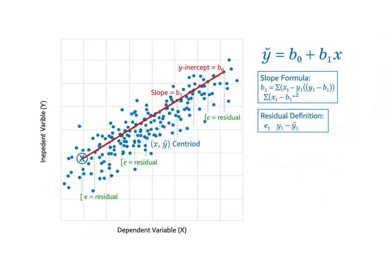
A regression line is a straight line fitted to paired numerical data to describe how the expected or predicted value of one variable changes as another variable changes. In simple least-squares regression, the fitted regression line is written as ŷ = b₀ + b₁x, where b₀ is the intercept and b₁ is the slope, while ŷ represents the response predicted by the line at a specified value of x. The slope measures the estimated change in the fitted response associated with a one-unit increase in the predictor, whereas the intercept gives the fitted response when x equals zero, provided that zero is a meaningful value within the relevant predictor range. Ordinary least squares chooses the line that minimizes the sum of squared vertical residuals between the observed responses and their fitted values, giving the regression line a precise mathematical definition rather than simply selecting a line that looks visually close to the points. The fitted line always passes through the point (x̄, ȳ) when an intercept is included, and its slope can be expressed through sums of cross-deviations, covariance and variance, or the correlation coefficient and standard deviations. A regression line can summarize association and generate predictions, but it does not by itself establish causation, guarantee accurate extrapolation, or prove that the relationship is truly linear.
The regression line is one of the foundational modeling tools within core statistics and the wider Statistics & Probability framework. Its estimates are calculated from sample data and therefore vary from sample to sample, which connects regression directly with sampling distributions and sample size when uncertainty around the fitted slope, intercept, or predictions must be quantified.
What Is a Regression Line?
A regression line is a fitted mathematical relationship between a predictor variable x and a response variable y. In simple regression, the relationship is represented by a straight line:
ŷ = b₀ + b₁x
where b₀ and b₁ are estimated from observed paired data.
The line describes the estimated conditional mean of y as x changes under the regression model. Individual observations generally do not lie exactly on the regression line because real data contain variation that is not explained by the predictor alone. Instead, each observation can be viewed as a fitted component plus a residual, with the regression line representing the systematic linear pattern and the residual representing the difference between an observed response and the fitted value.
A regression line therefore summarizes the central linear tendency of paired numerical data rather than attempting to pass through every individual point.
Regression Line Formula
The standard fitted regression line is:
ŷ = b₀ + b₁x
where:
- ŷ = predicted response
- x = predictor value
- b₀ = estimated intercept
- b₁ = estimated slope
The corresponding population model is commonly written:
Y = β₀ + β₁X + ε
where β₀ and β₁ are population parameters and ε represents random variation around the population line.
The fitted values:
b₀
and:
b₁
are statistics estimated from a sample.
This distinction is important because a sample regression line is not usually identical to the unknown population relationship. Different random samples can produce different slopes and intercepts even when they come from the same underlying population.
Regression Line Slope Formula
For paired observations:
(x₁,y₁), …, (xₙ,yₙ)
the least-squares slope is:
b₁ = Σ(xᵢ − x̄)(yᵢ − ȳ) / Σ(xᵢ − x̄)²
The numerator measures how x and y vary together around their sample means, while the denominator measures variation in x.
It is useful to define:
Sxy = Σ(xᵢ − x̄)(yᵢ − ȳ)
and:
Sxx = Σ(xᵢ − x̄)²
Then:
b₁ = Sxy/Sxx
provided:
Sxx > 0
If every x observation has the same value, then Sxx = 0 and a slope cannot be estimated because there is no predictor variation available to define a line.
Regression Line Intercept Formula
Once the slope is known, the intercept is:
b₀ = ȳ − b₁x̄
This formula guarantees that the fitted regression line passes through:
(x̄, ȳ)
because substituting:
x = x̄
gives:
ŷ = b₀ + b₁x̄
= ȳ − b₁x̄ + b₁x̄
= ȳ
Therefore, for ordinary least-squares simple regression with an intercept:
ŷ(x̄) = ȳ
This is one of the central geometric properties of the regression line.
Regression Line Example
Consider the paired observations:
| x | y |
|---|---|
| 1 | 2 |
| 2 | 3 |
| 3 | 5 |
| 4 | 4 |
| 5 | 6 |
We will calculate the least-squares regression line.
First find the means:
x̄ = (1 + 2 + 3 + 4 + 5)/5
x̄ = 3
and:
ȳ = (2 + 3 + 5 + 4 + 6)/5
ȳ = 4
Now calculate the deviations and cross-products.
| x | y | x − 3 | y − 4 | (x − 3)² | (x − 3)(y − 4) |
|---|---|---|---|---|---|
| 1 | 2 | −2 | −2 | 4 | 4 |
| 2 | 3 | −1 | −1 | 1 | 1 |
| 3 | 5 | 0 | 1 | 0 | 0 |
| 4 | 4 | 1 | 0 | 1 | 0 |
| 5 | 6 | 2 | 2 | 4 | 4 |
Therefore:
Sxx = 4 + 1 + 0 + 1 + 4
Sxx = 10
and:
Sxy = 4 + 1 + 0 + 0 + 4
Sxy = 9
The slope is:
b₁ = 9/10
b₁ = 0.9
The intercept is:
b₀ = 4 − 0.9(3)
b₀ = 4 − 2.7
b₀ = 1.3
Therefore, the regression line is:
ŷ = 1.3 + 0.9x
Interpreting the Slope
The slope is:
b₁ = 0.9
This means that for every one-unit increase in x, the fitted response increases by:
0.9 units
on average according to the estimated linear relationship.
If x increases from:
2 to 3
the fitted value increases by:
0.9
and the same fitted increase occurs when x rises from:
4 to 5.
That constant rate of change is what makes the model linear.
The slope describes the fitted conditional relationship, not necessarily a causal effect. A positive slope indicates positive linear association after defining the variables as modeled, but it does not prove that deliberately increasing x would cause y to rise by 0.9 units.
Interpreting the Intercept
The intercept is:
b₀ = 1.3
Therefore, the fitted equation predicts:
ŷ = 1.3
when:
x = 0
Whether that interpretation is useful depends on the meaning and observed range of x.
The sample contains:
x = 1 through 5
so x = 0 lies just outside the observed range. The mathematical intercept is necessary to position the fitted line, but a substantive interpretation at x = 0 should be cautious unless that predictor value is realistic and sufficiently supported by the application.
For some variables, x = 0 has direct meaning. For others, it can be physically impossible or far outside the available evidence.
Calculating Fitted Values
Using:
ŷ = 1.3 + 0.9x
the fitted response for:
x = 1
is:
ŷ = 1.3 + 0.9(1)
ŷ = 2.2
For:
x = 3
we obtain:
ŷ = 1.3 + 0.9(3)
ŷ = 4.0
For:
x = 5
we obtain:
ŷ = 1.3 + 0.9(5)
ŷ = 5.8
The fitted values for all observations are:
| x | Observed y | Fitted ŷ |
|---|---|---|
| 1 | 2 | 2.2 |
| 2 | 3 | 3.1 |
| 3 | 5 | 4.0 |
| 4 | 4 | 4.9 |
| 5 | 6 | 5.8 |
The line does not pass through every observed y value, nor is it intended to. It minimizes the total squared vertical discrepancy across the sample.
Residuals
A residual is:
eᵢ = yᵢ − ŷᵢ
For the example, the residual at:
x = 1
is:
e = 2 − 2.2
e = −0.2
At:
x = 3
the observed response is 5 while the fitted response is 4:
e = 5 − 4
e = 1
At:
x = 4
we have:
e = 4 − 4.9
e = −0.9
A positive residual means the observation lies above the regression line. A negative residual means it lies below the line.
Residual Table
For the full data set:
| x | y | ŷ | Residual e |
|---|---|---|---|
| 1 | 2 | 2.2 | −0.2 |
| 2 | 3 | 3.1 | −0.1 |
| 3 | 5 | 4.0 | 1.0 |
| 4 | 4 | 4.9 | −0.9 |
| 5 | 6 | 5.8 | 0.2 |
With an intercept included, ordinary least-squares residuals satisfy:
Σeᵢ = 0
For this example:
−0.2 − 0.1 + 1.0 − 0.9 + 0.2 = 0
This balancing property follows from the least-squares normal equations.
Why Least Squares Uses Squared Residuals
Ordinary least squares chooses b₀ and b₁ to minimize:
SSE = Σeᵢ²
or:
SSE = Σ(yᵢ − b₀ − b₁xᵢ)²
Squaring residuals prevents positive and negative errors from canceling, while also penalizing larger residuals more strongly.
For example:
residual = 2
contributes:
2² = 4
while:
residual = 6
contributes:
6² = 36
Therefore, the second residual is three times larger in absolute size but contributes nine times as much squared error.
This sensitivity is mathematically useful but also means unusual response observations can exert substantial influence on a least-squares regression line.
Sum of Squared Errors Example
For the fitted regression line:
ŷ = 1.3 + 0.9x
the residuals are:
−0.2, −0.1, 1.0, −0.9, 0.2
Square them:
0.04, 0.01, 1.00, 0.81, 0.04
Therefore:
SSE = 0.04 + 0.01 + 1.00 + 0.81 + 0.04
SSE = 1.90
No other straight line produces a smaller sum of squared vertical residuals for these five observations.
That minimizing property defines the least-squares regression line.
Why the Line Passes Through (x̄, ȳ)
The intercept formula is:
b₀ = ȳ − b₁x̄
Substitute x̄ into the fitted line:
ŷ = b₀ + b₁x̄
Then:
ŷ = ȳ − b₁x̄ + b₁x̄
so:
ŷ = ȳ
For the example:
x̄ = 3
ȳ = 4
and:
ŷ = 1.3 + 0.9(3)
= 4
Therefore, the point:
(3,4)
lies exactly on the fitted regression line.
This property holds for ordinary least-squares simple regression whenever an intercept is included.
Regression Slope and Covariance
The sample covariance is:
sxy = Σ(xᵢ − x̄)(yᵢ − ȳ)/(n − 1)
and the sample variance of x is:
sx² = Σ(xᵢ − x̄)²/(n − 1)
Dividing covariance by predictor variance gives:
b₁ = sxy/sx²
because the common denominator n − 1 cancels.
This expression shows that the regression slope depends on:
how x and y vary together
relative to:
how much x itself varies.
If covariance is positive, the fitted slope is positive. If covariance is negative, the fitted slope is negative, provided predictor variance is positive.
Regression Slope and Correlation
The sample correlation coefficient satisfies:
r = sxy/(sxsy)
Rearranging:
sxy = r sx sy
Substitute into:
b₁ = sxy/sx²
to obtain:
b₁ = r(sy/sx)
This formula connects the regression slope with correlation and scale.
It explains why correlation is unitless while slope has units. The ratio:
sy/sx
converts the standardized association r back into the measurement units of y per unit of x.
Why Slope Changes When Units Change
Suppose x is measured in meters and the regression slope is:
5 response units per meter.
If x is converted to centimeters:
1 meter = 100 centimeters
then a one-centimeter increase is only one-hundredth of a meter.
The numerical slope therefore becomes:
5/100
= 0.05 response units per centimeter.
The fitted relationship has not physically changed.
Only the measurement scale has changed.
Correlation would remain unchanged under positive linear unit conversion because it is standardized, while the regression slope changes with the units.
R-Squared
The coefficient of determination is:
R² = 1 − SSE/SST
where:
SST = Σ(yᵢ − ȳ)²
For the example, ȳ = 4, so:
SST = (2−4)² + (3−4)² + (5−4)² + (4−4)² + (6−4)²
SST = 4 + 1 + 1 + 0 + 4
SST = 10
Since:
SSE = 1.9
we obtain:
R² = 1 − 1.9/10
R² = 0.81
Therefore, approximately:
81%
of the sample variation in y around ȳ is accounted for by the fitted straight-line relationship in this least-squares decomposition.
R-Squared and Correlation in Simple Regression
In simple ordinary least-squares regression with an intercept:
R² = r²
For the example:
R² = 0.81
Therefore:
|r| = √0.81
= 0.9
Because the slope is positive:
r = 0.9
Thus, the data have a strong positive sample linear correlation.
This equality is specific to simple regression with an intercept. It should not be assumed automatically for every regression specification.
What R-Squared Does Not Mean
An R² of:
0.81
does not mean that x causes 81% of y.
It does not mean that 81% of individual observations are predicted correctly, nor does it guarantee that predictions will remain accurate in new data.
R² describes an in-sample variance decomposition relative to the sample mean under the fitted model.
A high R² can coexist with:
- biased sampling,
- confounding,
- nonlinear residual patterns,
- influential observations,
- poor extrapolation.
A low R² can also occur in scientifically meaningful systems where individual outcomes contain substantial natural variability.
Prediction From the Regression Line
Suppose we want the fitted response at:
x = 4.5
Using:
ŷ = 1.3 + 0.9x
we obtain:
ŷ = 1.3 + 0.9(4.5)
ŷ = 1.3 + 4.05
ŷ = 5.35
Therefore:
Predicted conditional mean ≈ 5.35
Because:
x = 4.5
lies within the observed range:
1 ≤ x ≤ 5
this is an interpolation.
The prediction still has uncertainty, but it is supported by predictor values on both sides of 4.5.
Extrapolation
Suppose the same regression line is used at:
x = 20
Then:
ŷ = 1.3 + 0.9(20)
ŷ = 19.3
The arithmetic is straightforward, but x = 20 lies far beyond the observed range of 1 through 5.
Nothing in the sample establishes that the same linear relationship continues that far.
This is extrapolation, and its reliability depends on substantive knowledge about the process rather than the regression equation alone.
A fitted regression line is evidence about the observed predictor region, not a guarantee of indefinite linear behavior.
Interpolation vs Extrapolation
Interpolation predicts within the observed predictor range.
Extrapolation predicts beyond it.
Both use the same equation, but they are not equally supported by data. During interpolation, nearby observed x values help constrain the fitted relationship. During extrapolation, the assumed linear form is projected into a region containing no direct observations.
Even a perfectly linear-looking sample can conceal curvature outside its observed range.
For that reason, extrapolated predictions should usually be identified explicitly.
Regression Line vs Polynomial Regression
A regression line has constant slope:
ŷ = b₀ + b₁x
By contrast, polynomial regression can include terms such as:
x²
and:
x³
so the slope changes across the predictor range.
For example:
ŷ = b₀ + b₁x + b₂x²
has derivative:
dŷ/dx = b₁ + 2b₂x
A polynomial should not be preferred merely because it can produce a higher in-sample R². Additional flexibility can overfit random variation.
The simpler regression line is preferable when a straight relationship adequately captures the systematic pattern and provides the stability or interpretation needed for the analysis.
Detecting Nonlinearity
A scatter plot should be examined before relying on a regression line. If the observations follow a clear curved pattern, a straight-line model can average across that curvature and produce misleading slopes or predictions.
Residual plots provide another diagnostic. If residuals are systematically positive in one part of the predictor range and negative in another, the regression line may have missed nonlinear structure.
For example, a U-shaped residual pattern can indicate that a quadratic term may be needed.
A line should therefore be selected because the relationship is adequately linear for the analytical purpose, not because linear regression is the easiest calculation.
Regression Line and Probability
A regression line does not assert that y is determined exactly by x. The statistical model contains a random component:
Y = β₀ + β₁X + ε
and probability describes the distribution of ε and therefore the uncertainty around the conditional mean.
A common assumption is:
E(ε|X) = 0
which implies:
E(Y|X=x) = β₀ + β₁x
Thus, the regression line represents the conditional expected response.
Individual observations vary around it because ε is not generally zero.
Conditional Mean
The population regression line is often interpreted as:
E(Y|X=x) = β₀ + β₁x
This is stronger and more precise than saying merely:
“y is related to x.”
It states that the conditional mean of Y changes linearly with X.
Suppose:
E(Y|X=x) = 10 + 2x
Then the expected response at:
x = 5
is:
20
An individual response at x = 5 could be:
16, 19, 25
or another value, depending on the error distribution.
The regression line describes the center of that conditional distribution rather than every realization.
Error Term vs Residual
The population error is:
εᵢ = Yᵢ − (β₀ + β₁Xᵢ)
It involves the unknown population regression parameters.
A sample residual is:
eᵢ = yᵢ − ŷᵢ
using estimated coefficients.
Errors are theoretical random quantities in the population model.
Residuals are observable after a model has been fitted to sample data.
Residuals are used to diagnose whether assumptions about the underlying errors appear reasonable.
The two concepts are closely related but should not be treated as identical.
Standard Error of the Regression
A common estimate of the residual standard deviation in simple regression is:
s = √[SSE/(n − 2)]
The denominator is:
n − 2
because two coefficients have been estimated:
b₀ and b₁.
For the worked example:
SSE = 1.9
n = 5
Therefore:
s = √(1.9/3)
s ≈ 0.796
This measures the typical residual scale in the original y units under the standard least-squares framework.
It is not the same quantity as R².
Standard Error of the Slope
Under the classical simple regression assumptions:
SE(b₁) = s/√Sxx
For the example:
s ≈ 0.796
and:
Sxx = 10
Therefore:
SE(b₁) ≈ 0.796/√10
SE(b₁) ≈ 0.252
The estimated slope is:
b₁ = 0.9
so the signal relative to its estimated standard error is:
0.9/0.252
≈ 3.58
This quantity forms the basis of a t-statistic for testing a population slope under the classical model.
Testing the Regression Slope
A common null hypothesis is:
H₀: β₁ = 0
against:
H₁: β₁ ≠ 0
The test statistic is:
t = (b₁ − 0)/SE(b₁)
For the example:
t ≈ 3.58
with:
df = n − 2
df = 3
The associated two-sided p-value is approximately:
p ≈ 0.037
under the standard t-test assumptions.
At:
α = 0.05
this provides evidence against a zero population slope.
It does not prove causation or guarantee that the linear model is correctly specified.
Confidence Interval for the Slope
A two-sided confidence interval for β₁ has the form:
b₁ ± t*SE(b₁)
where t* is the appropriate critical value for:
df = n − 2
For this small example:
df = 3
and the 95% t critical value is approximately:
3.182
Therefore:
0.9 ± 3.182(0.252)
which gives approximately:
0.9 ± 0.801
or:
(0.10, 1.70)
after rounding.
The interval is wide because the sample contains only five observations.
That illustrates how sample size affects uncertainty even when the fitted line appears strong.
Sample Size and the Regression Line
A regression line can be calculated from a very small number of observations, but mathematical calculability does not guarantee statistical precision.
With only a few data points, the slope can be highly sensitive to one observation and its standard error can be large. As suitable independent sample size increases across an informative predictor range, the line can generally be estimated more precisely, although the amount of information also depends on how x values are distributed.
Ten observations spread widely across the relevant predictor domain may provide more information about slope than ten observations clustered tightly around one x value.
Sample size and predictor variation both matter.
Why Predictor Spread Matters
The slope standard error contains:
Sxx = Σ(xᵢ − x̄)²
in its denominator.
Therefore, all else equal, greater predictor spread can provide more information about the slope.
Suppose all x observations lie between:
9.9 and 10.1.
It can be difficult to determine how y changes across a one-unit increase in x because the data contain almost no one-unit variation.
A sample covering a broader relevant x range can estimate the linear rate of change more effectively.
However, deliberately adding extreme x values solely to increase Sxx can create extrapolation, leverage, or design problems if those values are not scientifically relevant.
Sampling Distributions of Regression Estimates
If the study were repeated with new random samples from the same population, each sample would generally produce a different:
b₀
and:
b₁.
The distribution of those estimates across repeated samples is a sampling distribution.
The standard error of b₁ measures the estimated spread of its sampling distribution under the regression assumptions.
This is why uncertainty exists even though the fitted slope from one observed sample is a single number.
Inference concerns the behavior of the estimator across hypothetical repetitions, not merely the geometry of the observed line.
Confidence Interval for the Mean Response
Suppose we want the expected response at a particular predictor value x₀.
The fitted mean response is:
ŷ₀ = b₀ + b₁x₀
Its uncertainty is smallest near x̄ and generally grows as x₀ moves farther from the center of the observed predictor values.
Under the classical simple regression model:
SE(mean at x₀) = s√[1/n + (x₀ − x̄)²/Sxx]
A confidence interval for the mean response is then:
ŷ₀ ± t*SE(mean at x₀)
This interval describes uncertainty about the conditional mean, not the variation of an individual future observation.
Prediction Interval
For one new individual response at x₀, additional random error must be included.
The standard error becomes:
SE(prediction) = s√[1 + 1/n + (x₀ − x̄)²/Sxx]
The extra:
1
inside the square root represents individual outcome variation around the regression line.
Therefore, a prediction interval is wider than a confidence interval for the mean response at the same x₀.
This distinction is important because estimating an average response is easier than predicting exactly where one new individual observation will fall.
Assumption of Linearity
A regression line assumes that the conditional mean is adequately described by:
β₀ + β₁x
over the region being analyzed.
This does not require every observation to form a perfect straight line.
It requires the systematic mean relationship to be sufficiently linear for the intended purpose.
If the true relationship curves substantially, the estimated slope can become an average of differing local slopes and may obscure meaningful structure.
Plots of y against x and residuals against x or fitted values are useful for evaluating this assumption.
Constant Variance
A common classical assumption is:
Var(ε|X=x) = σ²
for all relevant x.
This is called homoscedasticity.
If residual variability increases as x increases, the conditional mean line can still be useful, but conventional standard errors and confidence intervals may need adjustment.
Changing variance is a separate issue from changing mean.
Adding curvature to the mean structure does not automatically solve heteroscedasticity.
Independence
Many simple regression procedures assume observations or errors are independent, conditional on the design.
This assumption can fail in:
- repeated measurements,
- time series,
- clustered samples,
- spatial data,
- family data.
If dependent observations are analyzed as though they were independent, conventional standard errors can be too small or otherwise inaccurate.
The fitted line itself may look reasonable while its reported inferential uncertainty is misleading.
Study design therefore matters as much as the equation.
Normality
Normally distributed errors are not required simply to compute b₀ and b₁ by least squares. They are more directly relevant to exact small-sample t and F inference under the classical model.
The relevant condition concerns the error distribution around the regression line at predictor values, not the marginal distribution of x itself.
Large samples can support approximate inference under broader conditions in many settings, but severe skewness, heavy tails, influential observations, dependence, or changing variance can still create important problems.
Normality should therefore be considered as part of a complete model, not a mechanical checkbox applied to the predictor.
Residual Quartiles
Residuals can be summarized using quartiles, particularly when analysts want a resistant description of the center and spread of regression errors.
Suppose residuals have:
Q₁ = −2.0
Median = 0.1
Q₃ = 2.4
Then:
IQR = 4.4
This gives useful information about the middle half of residuals.
However, quartiles discard the x-ordering of the residuals. A residual plot remains necessary to determine whether errors become systematically positive, negative, wider, or narrower as x changes.
Unusual Observations
A point can be unusual because its response is far from the fitted line, because its x value is far from the rest of the predictors, or because it has substantial influence on the fitted coefficients.
These properties are not identical.
A large residual identifies unusual y behavior relative to the current fit.
High leverage identifies unusual predictor position.
Influence describes how much the regression line changes when the observation is included or excluded.
A valid extreme-x observation can have high leverage while still lying almost exactly on the regression line.
Such a point should not automatically be removed.
How an Outlying Point Can Change a Regression Line
Suppose most observations lie near x values from 1 to 5, while one observation occurs at:
x = 50.
Because the slope calculation contains:
(xᵢ − x̄)
and squared x deviations, the distant observation can have substantial leverage.
If its y value follows the existing trend, it may strengthen evidence for the slope.
If it lies far away vertically, it can pull the line sharply toward itself.
This sensitivity makes scatter plots and influence diagnostics essential when interpreting a regression line.
Regression Toward the Mean
The phrase regression toward the mean is historically related to regression but should not be confused with the equation of a fitted regression line.
When two standardized variables have correlation less than 1 in magnitude, unusually extreme observations on one variable tend, on average, to be associated with less extreme standardized values on the other.
This is a statistical consequence of imperfect association, not a force that causes values to become average.
The fitted regression line can express this phenomenon under appropriate standardized variables, but the general concept is broader than merely calculating slope and intercept.
Reversing x and y Changes the Regression Line
The regression of y on x is generally not the inverse of the regression of x on y.
If we fit:
y on x
least squares minimizes vertical residuals in y.
If we fit:
x on y
it minimizes residuals in x.
Unless correlation is exactly:
±1
the two fitted lines do not simply invert one another.
Therefore, the choice of predictor and response should follow the scientific or predictive question rather than treating the variables as interchangeable.
Regression Line vs Correlation
Correlation measures the strength and direction of linear association on a standardized scale.
The regression line estimates a directional predictive relationship:
y from x.
Correlation is symmetric:
rxy = ryx
Regression is directional because predicting y from x is not the same optimization problem as predicting x from y.
Correlation contains no intercept and no measurement units.
A regression line contains both an intercept and a slope expressed in the variables’ units.
Regression Line vs Quartiles
Quartiles summarize one variable’s ordered distribution, whereas a regression line models the relationship between two numerical variables.
For example, quartiles can describe the spread of y without using x at all.
A regression line instead asks:
How does the fitted mean of y change as x changes?
The two can complement each other. Quartiles may summarize predictor, response, or residual distributions, while the regression line describes their linear relationship.
Regression Line vs Polynomial Regression
A regression line is appropriate when the systematic relationship is adequately linear over the region of interest. Polynomial regression becomes relevant when the conditional mean bends in a way that a constant slope cannot represent.
A quadratic model can change direction once, while a cubic model can represent even more complex curvature. That additional flexibility should be supported by residual patterns, validation performance, and substantive reasoning.
A straight regression line remains preferable when it captures the relationship adequately because it is generally easier to interpret, estimate, and extrapolate cautiously over short distances.
Regression Line and Causation
A positive regression slope does not by itself show that increasing x causes y to increase.
Suppose:
ŷ = 10 + 3x
The line establishes an estimated association in the observed data under the chosen model.
The relationship could arise because:
- x causes y,
- y influences x,
- a third variable affects both,
- the sample is selected in a particular way,
- both variables share a trend,
- the relationship is coincidental.
Causal interpretation requires design and assumptions that go beyond least-squares fitting.
Randomization, credible natural experiments, or well-justified causal identification strategies can provide information that a regression line alone cannot.
Prediction Does Not Require Causation
A regression line can be useful for prediction even when x does not cause y.
Suppose x is strongly associated with a future outcome because it serves as a useful marker.
The regression line may predict effectively while having no meaningful causal interpretation.
Prediction asks:
Does knowing x improve estimates of y?
Causal inference asks:
What would happen to y if x were intervened upon?
Those are different questions.
The fitted regression equation itself does not resolve the distinction.
Common Regression Line Mistakes
A common mistake is interpreting the slope as causal without a design that supports causation. A fitted association can be strong and statistically significant while being entirely noncausal.
Another error is assuming the regression line must pass through every data point. Least squares minimizes total squared residuals; it generally does not interpolate the observations.
A third mistake is interpreting the intercept when x = 0 is impossible or far outside the observed predictor range.
Another common problem is extrapolating a linear relationship far beyond the sample merely because the equation can produce a numerical answer.
Analysts also sometimes use R² as the only measure of model quality, ignoring nonlinearity, heteroscedasticity, dependence, and influential observations.
It is also incorrect to assume that a large p-value for slope proves no relationship exists; the sample may be too small or the relationship may be nonlinear.
Finally, reversing x and y produces a different least-squares problem and generally a different regression line.
How to Calculate a Regression Line Step by Step
Start with paired observations and identify which variable is the predictor x and which is the response y. Plot the data first so that a straight-line model is at least substantively plausible before performing the calculation.
Calculate the sample means:
x̄
and:
ȳ
Then calculate:
Sxx = Σ(xᵢ − x̄)²
and:
Sxy = Σ(xᵢ − x̄)(yᵢ − ȳ)
Use:
b₁ = Sxy/Sxx
followed by:
b₀ = ȳ − b₁x̄
The fitted regression line is:
ŷ = b₀ + b₁x
After fitting, calculate residuals:
eᵢ = yᵢ − ŷᵢ
and examine the residual pattern, influential observations, predictor range, and uncertainty before interpreting the line.
Full Worked Regression Line Example
Use:
| x | y |
|---|---|
| 1 | 2 |
| 2 | 3 |
| 3 | 5 |
| 4 | 4 |
| 5 | 6 |
The sample means are:
x̄ = 3
ȳ = 4
The cross-deviation total is:
Sxy = 9
The predictor squared-deviation total is:
Sxx = 10
Therefore:
b₁ = 9/10
= 0.9
and:
b₀ = 4 − 0.9(3)
= 1.3
The fitted regression line is:
ŷ = 1.3 + 0.9x
At:
x = 2.5
the fitted response is:
ŷ = 1.3 + 0.9(2.5)
= 3.55
At:
x = 4.5
the fitted response is:
ŷ = 5.35
The line passes through:
(3,4)
because that point is:
(x̄,ȳ)
and the fitted sample R² is:
0.81.
How to Report a Regression Line
A clear report should identify the fitted equation and interpret the slope in the variables’ units. For example:
“The fitted regression line was ŷ = 1.3 + 0.9x. Within the observed predictor range, the fitted response increased by approximately 0.9 units for each one-unit increase in x.”
If inferential analysis is relevant, add uncertainty rather than presenting the slope as exact:
“The estimated slope was 0.90 with a 95% confidence interval of approximately 0.10 to 1.70.”
The report should also state important limitations when necessary, such as a small sample, influential observations, nonlinear residuals, or predictions that extend beyond the observed x range.
A regression line is most useful when its equation, uncertainty, and domain of interpretation are communicated together.
Frequently Asked Questions About the Regression Line
What is a regression line?
A regression line is a fitted straight-line relationship used to describe or predict the conditional mean of a response variable from a numerical predictor.
What is the regression line formula?
ŷ = b₀ + b₁x
What does b₁ mean?
b₁ is the estimated slope. It gives the fitted change in y associated with a one-unit increase in x.
What does b₀ mean?
b₀ is the fitted intercept, representing the predicted response when x = 0.
Is the intercept always meaningful?
No. It may have little substantive meaning when x = 0 is impossible or far outside the observed predictor range.
What is the slope formula?
b₁ = Σ(xᵢ−x̄)(yᵢ−ȳ) / Σ(xᵢ−x̄)²
What is the intercept formula?
b₀ = ȳ − b₁x̄
Does the regression line pass through the sample means?
Yes. With an intercept included, the least-squares line passes through:
(x̄,ȳ)
What is a fitted value?
A fitted value is:
ŷᵢ = b₀ + b₁xᵢ
What is a residual?
eᵢ = yᵢ − ŷᵢ
It is the vertical difference between an observed response and its fitted value.
What does a positive residual mean?
The observed response lies above the regression line.
What does a negative residual mean?
The observed response lies below the regression line.
Why does least squares square residuals?
Squaring prevents positive and negative residuals from canceling and gives greater weight to larger errors.
What does least squares minimize?
SSE = Σ(yᵢ−ŷᵢ)²
Do regression residuals sum to zero?
For ordinary least-squares regression with an intercept:
Σeᵢ = 0
apart from numerical rounding.
What is R-squared?
R² = 1 − SSE/SST
It describes the fraction of sample variation around ȳ accounted for by the fitted regression model in the standard decomposition.
Is R² the same as correlation squared?
In simple ordinary least-squares regression with an intercept:
R² = r²
Does a high R² prove the model is correct?
No. A high R² can coexist with model misspecification, influential observations, confounding, or poor extrapolation.
What is the relationship between slope and correlation?
b₁ = r(sy/sx)
for simple regression.
Can a regression line have a negative slope?
Yes. A negative slope means the fitted response decreases as x increases.
What does a zero slope mean?
A slope of zero means the fitted straight line is horizontal, so the simple linear model predicts no change in the conditional mean of y as x changes.
Does a zero slope prove x and y are unrelated?
No. They could have a nonlinear relationship that a straight regression line does not capture.
What is interpolation?
Interpolation uses the regression line to predict at x values within the observed predictor range.
What is extrapolation?
Extrapolation predicts outside the observed range and can be much less reliable because the assumed linear pattern is unsupported by nearby observations.
What is the standard error of the regression?
In simple regression:
s = √[SSE/(n−2)]
under the conventional residual-variance estimator.
What is the standard error of the slope?
SE(b₁) = s/√Sxx
under the classical simple regression framework.
How is the slope tested?
A common statistic is:
t = b₁/SE(b₁)
for testing:
H₀: β₁ = 0
with:
df = n − 2
under the standard assumptions.
Does a significant slope prove causation?
No. Statistical evidence for association does not establish causal direction.
How does sample size affect a regression line?
Larger informative samples can reduce uncertainty around the fitted coefficients, but precision also depends on predictor variation, noise, dependence, and data quality.
Why does predictor spread matter?
The slope standard error depends inversely on:
√Sxx
so greater relevant spread in x can provide more information about the slope.
What is a sampling distribution of the slope?
It is the distribution of b₁ values that would arise across repeated comparable samples from the same population model.
What is the difference between a confidence interval and prediction interval?
A confidence interval describes uncertainty about the conditional mean response. A prediction interval includes additional variability for one future individual observation and is therefore wider.
Does x need to be normally distributed?
No. The predictor itself does not need a normal distribution for ordinary regression.
What does linearity mean?
It means the conditional mean of y is adequately represented by a straight-line function of x over the relevant predictor range.
What is homoscedasticity?
It is the assumption that conditional error variance is constant across predictor values.
Can regression be used when variance changes with x?
The fitted mean relationship can still be useful, but ordinary standard errors may require adjustment and the changing variance should be modeled or accounted for appropriately.
What is the difference between a regression line and polynomial regression?
A regression line has constant slope. Polynomial regression includes powers such as x² or x³ so the fitted slope can change with x.
Can quartiles be used with regression?
Yes. Quartiles can summarize predictor, response, or residual distributions, although they do not replace regression-specific diagnostic plots.
Why should residuals be plotted?
Residual plots can reveal curvature, heteroscedasticity, dependence, clusters, and unusual observations that a regression equation or R² alone can hide.
Is regression of y on x the same as regression of x on y?
No. The two models minimize errors in different variables and generally produce different fitted lines.
Can a regression line be useful without a causal relationship?
Yes. Association can support useful prediction even when x is not a causal driver of y.
What is the main rule when interpreting a regression line?
Interpret the slope within the observed predictor range, examine residuals and uncertainty, and do not treat association or a fitted equation as automatic evidence of causation.




