

Core Statistics: Complete Guide, Formulas & Examples

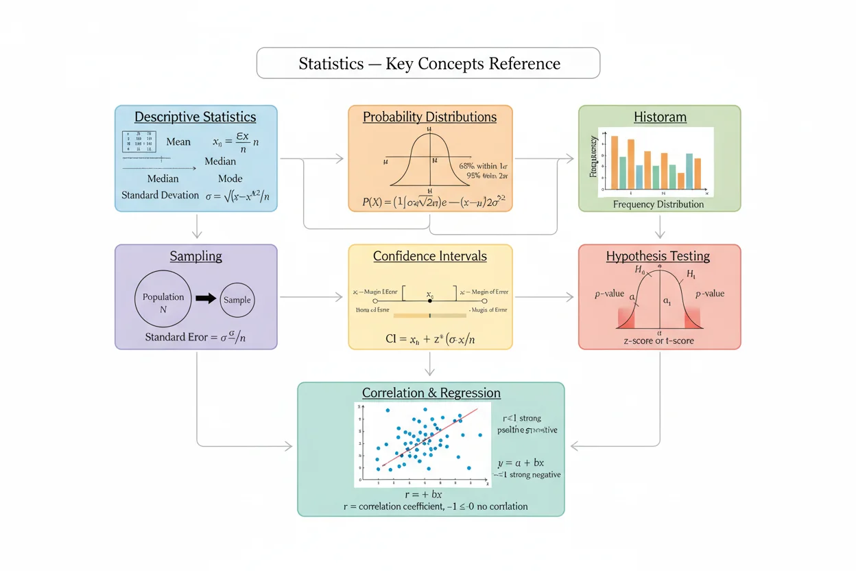
Core statistics provides the methods used to describe data, quantify uncertainty, compare groups, estimate population values, test claims, and model relationships between variables. A typical statistical analysis begins by identifying the population, sample, variables, and data types; continues with measures such as mean, variance, standard deviation, quartiles, and percentiles; then uses probability and sampling distributions to make inferences. Confidence intervals express estimation uncertainty, while hypothesis tests use statistics such as z, t, or chi-square to evaluate evidence against a stated null hypothesis. Correlation and regression quantify relationships between variables, while probability distributions describe how random outcomes are expected to behave. The correct method depends on the research question, data structure, assumptions, and whether the goal is description, estimation, testing, prediction, or probability calculation.
What Is Statistics?
Statistics is the discipline of collecting, organizing, analyzing, interpreting, and communicating information from data.
A useful distinction is between:
population — the complete group of interest
and:
sample — the observed subset used for analysis
The broad concepts and terminology behind variables, populations, samples, parameters, and statistics are introduced in Statistics Basics.
Descriptive and Inferential Statistics
Core statistics can be separated into two broad functions.
Descriptive methods summarize what the observed data look like.
Inferential methods use a sample to make statements about a larger population while accounting for uncertainty.
A dataset may therefore move from:
description
to:
probability modeling
to:
estimation or testing
without those stages being interchangeable.
Start With the Statistical Question
Before calculating anything, determine what is being asked.
Typical goals include:
What is a typical value?
How spread out are the observations?
How unusual is one observation?
How likely is an event?
Is there evidence of a difference?
How precisely has a population quantity been estimated?
Are two variables associated?
Can one variable predict another?
The question determines which statistical family is appropriate.
Mean
The arithmetic Mean of n observations is:
x̄ = Σxᵢ/n
For data:
4, 7, 9, 10
the mean is:
x̄ = 30/4
Therefore:
x̄ = 7.5
Mean is sensitive to unusually large or small observations, so it should be interpreted alongside information about the distribution.
Mean, Median, and Mode
The Mean, Median, Mode comparison helps distinguish three different notions of center.
The:
mean
uses every numerical value.
The:
median
is the middle ordered value.
The:
mode
is the most frequent value or category.
Their relative usefulness depends on distribution shape and data type.
Variance
Variance measures squared deviation from the center.
Population variance is:
σ² = Σ(xᵢ − μ)²/N
Sample variance is:
s² = Σ(xᵢ − x̄)²/(n−1)
The distinction between N and n−1 reflects whether the entire population or a sample is being described.
Standard Deviation
Standard Deviation is the square root of variance:
σ = √σ²
or for a sample:
s = √s²
Because it returns to the original measurement units, standard deviation is often easier to interpret than variance.
Mean and Variance Together
The Mean and Variance pair summarizes location and dispersion.
Two datasets can have the same mean but very different variability.
For example:
5, 5, 5, 5
and:
0, 0, 10, 10
both have mean:
5
but their spreads differ sharply.
A measure of center alone therefore does not fully describe numerical data.
Mean Absolute Deviation
Mean Absolute Deviation measures the average absolute distance from a chosen center, commonly the mean:
MAD = Σ|xᵢ − x̄|/n
Unlike variance, it does not square deviations.
That gives it a different interpretation of spread.
Quartiles
Quartiles divide ordered data into four broad sections.
Common notation is:
Q₁ = first quartile
Q₂ = median
Q₃ = third quartile
They help describe position and spread without relying heavily on extreme values.
Interquartile Range
The Interquartile Range is:
IQR = Q₃ − Q₁
It measures the width of the middle 50% of ordered observations.
Because it is based on quartiles, IQR is less sensitive to extreme values than the full range.
Outliers and the 1.5×IQR Rule
A common Outliers screening rule defines fences:
lower fence = Q₁ − 1.5(IQR)
upper fence = Q₃ + 1.5(IQR)
Observations outside these fences are flagged as potential outliers.
A flagged value is not automatically an error; it is a value that deserves closer interpretation.
Percentiles
Percentiles describe relative position in an ordered distribution.
A value at approximately the 80th percentile is at or above roughly 80% of the reference observations under the percentile convention being used.
Percentiles communicate rank rather than absolute distance between values.
Probability
Probability quantifies uncertainty.
For equally likely elementary outcomes:
P(A) = favorable outcomes / total outcomes
More generally:
0 ≤ P(A) ≤ 1
and:
P(Aᶜ) = 1 − P(A)
Probability provides the mathematical foundation for distributions, sampling, confidence intervals, and hypothesis testing.
Conditional Probability
The probability of A given B is:
P(A|B) = P(A ∩ B)/P(B)
provided:
P(B) > 0
Conditional probability changes the reference set from all possible outcomes to those for which B has occurred.
This idea is central to statistical updating and dependence.
Bayes’ Theorem
Bayes’ Theorem reverses a conditional probability:
P(A|B) = P(B|A)P(A)/P(B)
At a high level, it combines:
prior information
with:
evidence
to obtain an updated probability.
The detailed interpretation depends heavily on the events or statistical model involved.
Odds and Probability
The Odds Formats relationship converts between probability and odds.
If event probability is p:
odds in favor = p/(1−p)
Conversely, if decimal odds are interpreted under a specified convention, implied probability can be recovered from the appropriate reciprocal relationship.
Probability and betting-style odds express related information in different forms.
Random Variables and Distributions
A probability distribution describes how probability is allocated across the possible values of a random variable.
Different distributions model different mechanisms.
Important questions include whether the variable is:
discrete or continuous
whether trials are:
independent
and whether the probability structure remains:
constant or changing
These features determine which distribution is appropriate.
Binomial Distribution
The Binomial Distribution models the number of successes in n independent Bernoulli trials with constant success probability p.
Its probability mass function is:
P(X=k) = C(n,k)pᵏ(1−p)ⁿ⁻ᵏ
Typical conditions include:
fixed number of trials
two outcomes per trial
constant p
independent trials
The specialist distribution page develops its PMF and CDF in detail.
Binomial Probability
The Binomial Probability page focuses on calculating probabilities such as:
exactly k successes
at most k successes
at least k successes
within the binomial model.
This distinction matters because defining a distribution and evaluating a specific cumulative event are related but not identical tasks.
Geometric Distribution
The Geometric Distribution models waiting for the first success in repeated independent trials with constant success probability p.
One common form is:
P(X=k) = (1−p)ᵏ⁻¹p
for:
k = 1,2,3,…
Its question is about when the first success occurs, rather than how many successes appear in a fixed number of trials.
Negative Binomial Distribution
The Negative Binomial family extends the waiting-time idea to a specified number of successes.
Depending on convention, the random variable may count:
trials until the rth success
or:
failures before the rth success
Always confirm the definition before applying a formula.
Poisson Distribution
The Poisson Distribution models event counts over a specified interval under an appropriate rate-based process.
Its probability mass function is:
P(X=k) = e⁻λ λᵏ/k!
where:
λ = expected count in the interval
The model is often used for counts rather than binary trial totals.
Normal Distribution
The Normal Distribution is a continuous bell-shaped distribution characterized by:
mean μ
and:
standard deviation σ
Its symmetry and standardized form make it central to many statistical procedures.
Not every dataset is normal, so model assumptions should not be inferred solely from the familiarity of the bell curve.
Z-Score
A Z-Score standardizes an observation:
z = (x − μ)/σ
A positive z-score lies above the mean.
A negative one lies below.
Its magnitude expresses distance from the mean in units of standard deviation.
Z-Score Example
Suppose:
x = 85
μ = 70
σ = 10
Then:
z = (85−70)/10
Therefore:
z = 1.5
The observation lies:
1.5 standard deviations
above the mean.
Sampling
Most statistical inference is based on samples rather than complete populations.
A good sampling process aims to produce data that meaningfully represent the target population.
Bias in how observations are selected can undermine later calculations even when the formulas themselves are applied correctly.
Statistical inference cannot automatically repair a fundamentally unrepresentative sample.
Sampling Distributions
Sampling Distributions describe the distribution of a statistic across repeated samples.
Examples include distributions of:
sample means
sample proportions
sample variances
This concept connects observed sample statistics with probability models used for estimation and testing.
Standard Error
A standard error describes the variability of a statistic across repeated samples.
For a sample mean under the usual independent-observation framework with population standard deviation σ:
SE(x̄) = σ/√n
When σ is unknown, a sample-based estimate is often used in appropriate procedures.
Increasing n generally reduces standard error at a square-root rate.
Sample Size
Sample Size affects precision and statistical power.
Because many standard errors contain:
1/√n
doubling sample size does not halve sampling uncertainty.
To roughly halve a standard error under the same assumptions, sample size generally needs to be multiplied by about:
4
The exact planning formula depends on the parameter, design, desired precision, confidence level, and assumptions.
Confidence Intervals
Confidence Intervals provide an estimate together with a margin reflecting sampling uncertainty.
A broad structure is:
estimate ± critical value × standard error
The exact critical value and standard-error formula depend on the model and parameter.
Confidence intervals communicate a range of plausible parameter values under the procedure’s assumptions.
Confidence Level
The Confidence Level describes the long-run coverage target of a confidence-interval procedure.
Common levels include:
90%
95%
99%
A higher confidence level generally requires a wider interval when the data and method are otherwise unchanged.
Critical Values
Critical Values mark threshold positions in reference distributions.
Common families include:
z critical values
t critical values
chi-square critical values
Their value depends on the selected tail probability, confidence level or significance level, and sometimes degrees of freedom.
Hypothesis Testing
A statistical hypothesis test generally begins with:
null hypothesis H₀
and:
alternative hypothesis H₁
A test statistic summarizes how far the observed data depart from what H₀ predicts.
That statistic is interpreted through an appropriate reference distribution.
The result is evidence about compatibility with H₀, not a direct proof that one hypothesis is absolutely true.
P-Values
A P-Values calculation measures how incompatible the observed result, or something at least as extreme under the test definition, is with the null model.
A small p-value indicates that the observed data would be relatively unusual under H₀.
It does not directly mean:
probability that H₀ is true
nor does it measure the size or practical importance of an effect.
Significance Level
A hypothesis test often specifies:
α
before examining the result.
A common rule is to reject H₀ when:
p ≤ α
under the chosen procedure.
The significance level controls a long-run Type I error rate under the test’s assumptions; it should not be interpreted as a universal measure of scientific importance.
z-Test
A z-Test uses a z reference distribution under conditions appropriate to the parameter and sampling model.
A generic standardized form is:
z = (estimate − null value)/standard error
The correct numerator and standard-error expression depend on whether the test concerns a mean, proportion, difference, or another quantity.
t-Test
A t-Test uses the t distribution, commonly when estimating or testing mean-related quantities with unknown population variability under appropriate conditions.
The exact procedure differs for:
one-sample tests
paired tests
independent-sample tests
The degrees of freedom and standard-error calculation must match the design.
Chi-Square Methods
The Chi-Square family appears in procedures involving categorical counts and variance-related inference.
A common count-based statistic has the structure:
χ² = Σ(O−E)²/E
where:
O = observed count
E = expected count
The relevant chi-square procedure determines how expected counts and degrees of freedom are obtained.
ANOVA
ANOVA is used to analyze differences among multiple group means under a specified model.
Its central comparison is between:
variation explained by group differences
and:
variation within groups
The resulting F statistic can indicate evidence that not all modeled group means are equal.
A significant omnibus result does not by itself identify every pair of groups that differs.
Correlation
The Correlation Coefficient measures the direction and strength of a specified type of association, commonly linear association for Pearson’s r.
Its range is:
−1 ≤ r ≤ 1
A value near:
+1
indicates strong positive linear association.
Near:
−1
indicates strong negative linear association.
Near zero indicates weak linear association, though nonlinear relationships may still exist.
Correlation Does Not Establish Causation
A strong association can arise from:
direct causation
reverse causation
confounding variables
selection effects
or other mechanisms.
Statistical association alone does not identify which causal explanation is correct.
Study design and subject-matter reasoning remain essential.
Covariance
Covariance measures how two variables vary together.
A positive covariance indicates that above-average values of one variable tend to accompany above-average values of the other.
A negative covariance indicates the opposite tendency.
Unlike correlation, covariance depends on the measurement scales of the variables.
Regression
Regression models describe how an outcome changes in relation to one or more predictors.
The simplest Linear Regression model is often written:
ŷ = b₀ + b₁x
where:
b₀ = intercept
b₁ = estimated slope
The model’s usefulness depends on fit, assumptions, prediction range, and the question being asked.
Regression Line
The Regression Line represents the fitted linear relationship between predictor x and outcome y.
Its slope describes the estimated change in predicted y for a one-unit increase in x.
A fitted line should not be extrapolated far outside the observed predictor range without strong justification.
Polynomial Regression
Polynomial Regression allows curvature by incorporating powers such as:
x²
x³
and higher terms.
For example:
ŷ = b₀ + b₁x + b₂x²
can model a curved relationship that a straight line cannot capture.
Higher polynomial order is not automatically better; complexity can reduce interpretability and increase overfitting risk.
Exponential Regression
Exponential Regression models relationships that change multiplicatively, often using a form such as:
y = abˣ
or:
y = aeᵏˣ
depending on notation.
The model is appropriate only when the data-generating pattern supports exponential behavior.
Logarithmic Regression
Logarithmic Regression uses a form such as:
y = a + b ln x
for:
x > 0
It can represent relationships where changes are rapid initially and then progressively smaller.
Its domain restriction is essential because the logarithm is not defined for nonpositive real x.
Choosing a Regression Model
A model should be selected based on:
data pattern
residual behavior
domain knowledge
predictive purpose
interpretability
not simply by whichever equation produces the largest apparent fit statistic on the observed sample.
Linear, polynomial, exponential, and logarithmic models capture different structures.
Statistical Model Assumptions
Many methods rely on assumptions concerning factors such as:
independence
sampling design
distributional shape
variance structure
linearity
expected cell counts
or:
measurement scale
The assumptions differ by procedure.
A method can produce a numerical answer even when its assumptions are inappropriate, so calculation alone is not enough.
Parameter Versus Statistic
A parameter describes a population.
Examples include:
μ = population mean
σ = population standard deviation
A statistic is calculated from a sample.
Examples include:
x̄ = sample mean
s = sample standard deviation
Inferential statistics uses sample statistics to learn about unknown population parameters.
Point Estimates
A point estimate gives one numerical estimate of a parameter.
For example:
x̄
may estimate:
μ
A confidence interval adds a range reflecting sampling uncertainty around an estimate.
Point estimates are concise, but they do not communicate precision by themselves.
Effect Size and Statistical Significance
A statistically detectable result may still be small in practical terms.
Likewise, a potentially important effect can fail to reach a conventional significance threshold when data are limited or noisy.
Interpretation should therefore consider:
effect magnitude
uncertainty
study design
practical context
rather than relying only on a p-value.
Describing a Dataset Before Testing It
Before inferential calculations, inspect the observed data.
Useful summaries include:
center
spread
distribution shape
missing observations
unusual values
group sizes
relationships among variables
This stage can reveal errors or model problems that a later hypothesis test would not automatically detect.
A Compact Statistical Workflow
A sound core statistics workflow can be summarized as:
define the question and population
understand the variables and data structure
inspect and summarize the sample
choose an appropriate probability or statistical model
check relevant assumptions
calculate estimates, intervals, tests, or predictions
interpret the magnitude and uncertainty in context
The numerical result is one part of the analysis rather than the entire conclusion.
Example: Describing a Small Dataset
Suppose the observations are:
4, 6, 6, 8, 11
The mean is:
x̄ = 35/5
Therefore:
x̄ = 7
The median is:
6
The range is:
11 − 4 = 7
These simple summaries already reveal more about the dataset than any one statistic alone.
Further analysis would depend on what question the data are meant to answer.
Example: Standardizing a Value
Suppose:
μ = 100
σ = 15
and:
x = 130
Then:
z = (130−100)/15
Therefore:
z = 2
The observation lies two standard deviations above the stated mean.
Whether that is rare depends on the distribution being modeled.
Example: Probability Complement
Suppose an event has:
P(A) = 0.72
Then:
P(Aᶜ) = 1 − 0.72
Therefore:
P(Aᶜ) = 0.28
This simple complement relationship is used throughout probability calculations.
Example: Basic Confidence-Interval Structure
Suppose a procedure produces:
estimate = 50
margin of error = 4
Then the interval is:
50 ± 4
or:
[46,54]
The statistical meaning of that interval depends on how the margin of error was obtained and whether the method’s assumptions are satisfied.
Example: Correlation Interpretation
Suppose a calculated Pearson correlation is:
r = −0.82
This indicates a strong negative linear association in the observed data.
It does not by itself establish:
causation
nor does it tell whether a nonlinear pattern is present.
A scatter plot and the data context remain important.
Data Quality Comes Before Formula Choice
A sophisticated statistical formula cannot compensate for:
incorrect measurements
biased sampling
inconsistent definitions
duplicated observations
missing-data problems
or:
inappropriate variable coding
Statistical reasoning therefore begins with the data-generating process, not with a calculator.
Sample Size Is Not the Only Quality Measure
A large sample can improve precision, but a large biased sample can still provide a precisely wrong picture of the target population.
Sample size should therefore be evaluated together with:
sampling method
measurement quality
independence
representativeness
and:
missingness
Probability Models Are Simplifications
A distribution is a mathematical model of uncertainty.
Real observations do not need to resemble a formula perfectly for a model to be useful, but the approximation must be reasonable for the question being asked.
Model choice should follow the mechanism and data structure rather than familiarity alone.
Common Core Statistics Mistakes
A common mistake is treating mean, median, and mode as interchangeable.
Another is using sample and population variance formulas without distinguishing:
n−1
from:
N
Do not interpret correlation as proof of causation.
A p-value is not the probability that the null hypothesis is true.
A confidence level is not the probability that one already-computed fixed interval contains the parameter under the standard frequentist interpretation.
Do not select a probability distribution without checking its conditions.
Avoid assuming that every dataset is normally distributed.
When fitting regression models, inspect whether the chosen functional form makes sense.
Finally, report uncertainty and context rather than presenting a statistic as a self-explanatory conclusion.
Frequently Asked Questions
What is core statistics?
Core statistics is the set of foundational methods used to summarize data, model uncertainty, estimate population quantities, test hypotheses, and analyze relationships.
What is the difference between a population and a sample?
A population is the complete group of interest; a sample is the observed subset used for analysis.
What is the mean formula?
x̄ = Σxᵢ/n
Also, What is sample variance?
s² = Σ(xᵢ−x̄)²/(n−1)
What is standard deviation?
The square root of variance:
s = √s²
What is a z-score?
z = (x−μ)/σ
It expresses an observation’s distance from the mean in standard-deviation units.
What is probability?
A numerical measure of uncertainty between:
0 and 1
What is a confidence interval?
A range produced by an estimation procedure to communicate uncertainty about a population parameter.
What is a p-value?
A measure of how incompatible the observed result is with the null model under the specified test.
What is correlation?
A measure of association between variables; Pearson’s r specifically measures linear association.
What is regression?
A family of methods for modeling an outcome in relation to one or more predictors.
What is ANOVA used for?
It analyzes group-mean variation under an appropriate multi-group model.
What is the purpose of a sampling distribution?
It describes how a statistic varies across repeated samples and provides a basis for standard errors, intervals, and tests.
Why does sample size matter?
Larger samples can reduce sampling uncertainty and increase power, although design quality remains essential.
How do you choose a statistical method?
Start with the research question, variable types, study design, data structure, assumptions, and whether the objective is description, estimation, testing, probability, or prediction.
What should be checked before interpreting a statistical result?
Check data quality, sampling design, assumptions, effect magnitude, uncertainty, and whether the selected method actually addresses the intended question.




