

Standard Deviation: Definition, Formula & Example

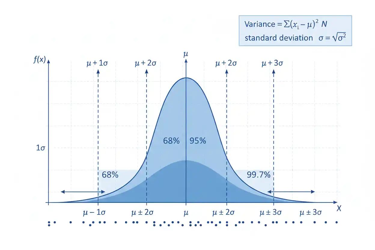
Standard deviation is a measure of dispersion that describes how far observations typically lie from their mean, expressed in the same units as the original data. A small standard deviation indicates that values are concentrated relatively close to the mean, whereas a large standard deviation indicates greater spread around that center. The calculation begins by measuring each observation’s deviation from the mean, squaring those deviations so positive and negative differences do not cancel, averaging the squared deviations according to either a population or sample formula, and finally taking the square root. This makes standard deviation the square root of variance and explains why the two measures contain closely related information even though they are expressed in different units. Standard deviation is fundamental throughout statistics because it appears in standardized scores, sampling distributions, confidence intervals, regression models, hypothesis tests, probability distributions, and measures of statistical uncertainty. However, its interpretation depends strongly on distribution shape, because a single standard deviation does not by itself reveal skewness, multimodality, extreme observations, or whether the mean is an appropriate center for the data.
Standard deviation is one of the foundational measures within core statistics and the wider Statistics & Probability framework. It connects elementary descriptive ideas from statistics basics with inferential concepts such as standard errors, test statistics, and the variability of estimators across repeated samples.
What Is Standard Deviation?
Standard deviation measures the spread of numerical observations around their arithmetic mean. It answers a different question from the mean itself: the mean describes where the data are centered arithmetically, while standard deviation describes how dispersed the observations are around that center.
Consider two data sets:
A: 48, 49, 50, 51, 52
B: 10, 30, 50, 70, 90
Both have mean:
50
Yet their spreads are dramatically different. Data set A is tightly concentrated around 50, whereas data set B extends far from the mean in both directions. Standard deviation captures that difference even though the means are identical.
For data set A, the population standard deviation is approximately:
1.414
For data set B, it is approximately:
28.284
The larger value reflects the much greater dispersion in B.
Standard Deviation Formula
For a population containing N observations, population standard deviation is:
σ = √[Σ(xᵢ − μ)²/N]
where:
- σ = population standard deviation
- xᵢ = individual population observation
- μ = population mean
- N = population size
For a sample containing n observations, sample standard deviation is:
s = √[Σ(xᵢ − x̄)²/(n − 1)]
where:
- s = sample standard deviation
- xᵢ = sample observation
- x̄ = sample mean
- n = sample size
The major structural difference is the denominator:
Population → N
Sample estimator → n − 1
The choice is not an arbitrary formatting convention. The sample formula with n − 1 is designed so that the corresponding sample variance is unbiased for the population variance under the usual independent-identically-distributed sampling framework.
Population Standard Deviation
Use the population formula when the data represent the entire population whose dispersion is being described.
Suppose the complete population is:
2, 4, 6, 8, 10
The population mean is:
μ = (2 + 4 + 6 + 8 + 10)/5
μ = 6
Calculate deviations:
2 − 6 = −4
4 − 6 = −2
6 − 6 = 0
8 − 6 = 2
10 − 6 = 4
Square them:
16, 4, 0, 4, 16
Their sum is:
40
The population variance is:
σ² = 40/5
σ² = 8
Therefore, the population standard deviation is:
σ = √8
σ ≈ 2.828
Thus, the observations have a population standard deviation of approximately 2.83 units around their mean of 6.
Sample Standard Deviation
Suppose instead that:
2, 4, 6, 8, 10
are a random sample from a larger population.
The sample mean is still:
x̄ = 6
and the sum of squared deviations remains:
40
However, sample variance is:
s² = 40/(5 − 1)
s² = 10
Therefore:
s = √10
s ≈ 3.162
The sample standard deviation is approximately:
3.16
The difference between 2.83 and 3.16 comes from the purpose of the calculation. The first describes the spread of those five values as the complete population, while the second uses them to estimate variability in a larger population.
Why Does Sample Standard Deviation Use n − 1?
The sample mean x̄ is estimated from the same observations used to calculate deviations, which imposes a constraint:
Σ(xᵢ − x̄) = 0
Once n − 1 deviations are known, the final deviation is determined automatically because all deviations must sum to zero. The deviations therefore have:
n − 1
degrees of freedom.
More importantly, dividing the squared-deviation sum by n tends to underestimate population variance when x̄ is substituted for the unknown μ. Dividing by:
n − 1
corrects this bias for the variance estimator under standard random-sampling assumptions.
This correction is known as Bessel’s correction.
Variance and Standard Deviation
Variance is the average squared deviation from the mean under the relevant population or sample formula, while standard deviation is the square root of that variance.
For a population:
σ² = Σ(xᵢ − μ)²/N
and:
σ = √σ²
For a sample:
s² = Σ(xᵢ − x̄)²/(n − 1)
and:
s = √s²
Because variance squares the deviations, its units are also squared. If observations are measured in meters, variance is expressed in:
meters²
Standard deviation takes the square root and returns to:
meters
This is one reason standard deviation is usually easier to interpret directly.
Why Deviations Are Squared
If ordinary deviations were simply added:
Σ(xᵢ − x̄)
the result would equal:
0
whenever x̄ is the arithmetic mean.
Positive deviations above the mean and negative deviations below it cancel exactly.
Squaring solves this problem:
(xᵢ − x̄)² ≥ 0
for every observation.
It also places greater weight on observations far from the mean. A deviation of 10 contributes:
10² = 100
whereas a deviation of 2 contributes:
2² = 4
so the first deviation is five times as large in absolute magnitude but contributes twenty-five times as much to the squared-deviation total.
This sensitivity is both an important feature and an important limitation of standard deviation.
Step-by-Step Standard Deviation Example
Consider the sample:
4, 7, 8, 10, 11
First calculate the sample mean:
x̄ = (4 + 7 + 8 + 10 + 11)/5
x̄ = 40/5
x̄ = 8
Now calculate deviations:
| x | x − x̄ | (x − x̄)² |
|---|---|---|
| 4 | −4 | 16 |
| 7 | −1 | 1 |
| 8 | 0 | 0 |
| 10 | 2 | 4 |
| 11 | 3 | 9 |
The squared deviations sum to:
16 + 1 + 0 + 4 + 9 = 30
Because these observations are being treated as a sample:
s² = 30/(5 − 1)
s² = 7.5
Therefore:
s = √7.5
s ≈ 2.739
The sample standard deviation is approximately:
2.74
Interpreting the Example
The sample mean is:
8
and the standard deviation is approximately:
2.74
This tells us that the observations have a characteristic spread of roughly a few units around the mean, but it should not be interpreted as saying every observation lies exactly 2.74 units from 8. The actual absolute deviations are:
4, 1, 0, 2, 3
Standard deviation is derived from the root mean square structure of deviations, not from the ordinary arithmetic mean of absolute distances.
It summarizes dispersion in one number rather than describing each individual distance.
Standard Deviation Is Never Negative
Variance is built from squared deviations:
(xᵢ − μ)² ≥ 0
Therefore:
Variance ≥ 0
and consequently:
Standard deviation ≥ 0
A negative standard deviation is mathematically impossible.
If all observations are identical, every deviation is zero and:
Standard deviation = 0
Otherwise, standard deviation is positive.
Zero Standard Deviation
Consider:
7, 7, 7, 7, 7
The mean is:
7
Every deviation is:
7 − 7 = 0
Therefore:
σ² = 0
and:
σ = 0
A zero standard deviation means there is no numerical variation in the data under consideration. Every observation is exactly equal to the mean.
It does not mean the mean itself is zero.
Standard Deviation and the Mean
Standard deviation measures dispersion around the arithmetic mean, so the mean is built directly into its calculation. If a different measure of center were used, the resulting dispersion statistic would generally be different.
The arithmetic mean has a special least-squares property: it minimizes the sum:
Σ(xᵢ − c)²
over all possible constants c.
Thus, squared deviations around the mean are smaller in total than squared deviations around any other fixed center.
This connection helps explain why means, variances, standard deviations, and least-squares regression are mathematically linked.
Standard Deviation vs Mean Absolute Deviation
Mean absolute deviation uses absolute rather than squared distances.
A general form around the mean is:
MAD_mean = Σ|xᵢ − x̄|/n
Standard deviation instead relies on:
√[average squared deviations]
Because squaring emphasizes large deviations more strongly than absolute values, standard deviation is generally more sensitive to extreme observations.
Neither measure is universally superior. Standard deviation is especially important because of its mathematical role in probability theory and inference, while absolute-deviation measures can offer greater resistance to extremes.
Standard Deviation vs Interquartile Range
The interquartile range measures central spread:
IQR = Q₃ − Q₁
Standard deviation uses every observation through squared deviations from the mean.
Consequently, the IQR is usually much more resistant to a few extreme observations, whereas standard deviation can increase sharply when even one value lies far from the mean.
For symmetric, light-tailed data, mean and standard deviation often provide an efficient and familiar summary. For highly skewed data or distributions containing legitimate extreme values, median and IQR may communicate central location and spread more robustly.
The choice should follow the shape and analytical objective rather than a rigid rule.
Standard Deviation and Outliers
Suppose:
10, 11, 12, 13, 14
The population mean is:
12
and population standard deviation is approximately:
1.414
Now replace 14 with:
100
The data become:
10, 11, 12, 13, 100
The mean rises dramatically to:
29.2
and the population standard deviation becomes approximately:
35.41
One extreme observation affects standard deviation in two ways: its own squared deviation is enormous, and it also moves the mean, changing the deviations of every other observation.
Standard deviation is therefore not robust to extreme values.
A Large Standard Deviation Is Not Automatically Bad
Whether standard deviation is “large” depends on the scale and application.
A standard deviation of:
10
could be enormous if observations typically lie around 5, but relatively small if observations lie around 100,000.
The units matter.
The acceptable amount of variability also depends on the process being studied. A manufacturing specification may require extremely low dispersion, while naturally heterogeneous human measurements can legitimately exhibit much greater spread.
Standard deviation should therefore be interpreted relative to the measurement scale, mean when appropriate, expected process behavior, and substantive consequences of variability.
Coefficient of Variation
For positive ratio-scale data with a meaningful nonzero mean, relative variability is sometimes summarized by the coefficient of variation:
CV = σ/μ
or, for sample quantities:
CV = s/x̄
It is often expressed as a percentage:
CV% = 100(s/x̄)
Suppose:
x̄ = 100
and:
s = 15
Then:
CV = 15/100
= 0.15
or:
15%
This can help compare variability across measurements with different means or units when the scale supports ratio comparisons.
The coefficient of variation is not appropriate for every measurement scale, particularly when zero is arbitrary or the mean is near zero.
Standard Deviation Under Addition of a Constant
Suppose every observation is transformed by:
Y = X + c
Adding a constant shifts every observation and the mean by the same amount, so deviations from the mean do not change.
Therefore:
SD(Y) = SD(X)
For example, if:
10, 12, 14
becomes:
110, 112, 114
after adding 100, the center changes but the spread remains identical.
Standard deviation is therefore invariant to translations of the measurement scale.
Standard Deviation Under Multiplication
Suppose:
Y = aX
Then:
SD(Y) = |a|SD(X)
If every observation is doubled, standard deviation doubles.
If every observation is divided by 100, standard deviation is divided by 100.
The absolute value appears because standard deviation cannot be negative.
For a full linear transformation:
Y = aX + b
the rule is:
SD(Y) = |a|SD(X)
The shift b affects location but not dispersion.
Standard Deviation and z-Scores
A z-score expresses an observation’s distance from the mean in units of standard deviation.
For a population:
z = (x − μ)/σ
Suppose:
μ = 100
σ = 15
and:
x = 130
Then:
z = (130 − 100)/15
z = 2
The observation lies:
2 standard deviations above the mean.
If:
x = 70
then:
z = (70 − 100)/15
z = −2
which means two standard deviations below the mean.
Standardization makes values from different scales more directly comparable in terms of relative position.
Standardizing a Distribution
If X has mean μ and positive standard deviation σ, define:
Z = (X − μ)/σ
Then:
E(Z) = 0
and:
SD(Z) = 1
Standardization shifts the center to zero and rescales dispersion to one.
It does not necessarily make the distribution normal.
A skewed distribution remains skewed after a positive linear standardization; its numerical center and scale change, but its overall shape is preserved.
Standard Deviation and the Normal Distribution
When a population follows a normal distribution:
X ~ N(μ, σ²)
standard deviation has an especially clear probability interpretation because normal distributions have a fixed shape determined by μ and σ.
Approximately:
68.27%
of observations lie within:
μ ± 1σ
Approximately:
95.45%
lie within:
μ ± 2σ
Approximately:
99.73%
lie within:
μ ± 3σ
This is commonly called the empirical 68–95–99.7 rule.
These percentages apply specifically to a normal distribution and should not be treated as universal rules for arbitrary data.
Example of the 68–95–99.7 Rule
Suppose:
X ~ N(100, 15²)
Then approximately 68.27% of observations lie between:
100 − 15 = 85
and:
100 + 15 = 115
Approximately 95.45% lie between:
70 and 130
and approximately 99.73% lie between:
55 and 145
These statements follow from the normal distribution’s shape, not from standard deviation alone.
A highly skewed distribution with the same mean and standard deviation can have very different percentages inside these intervals.
Chebyshev’s Inequality
For distributions with finite mean and variance, Chebyshev’s inequality provides a much more general statement that does not require normality.
For:
k > 1
at least:
1 − 1/k²
of probability lies within k standard deviations of the mean.
For:
k = 2
at least:
1 − 1/4 = 0.75
or:
75%
lies within two standard deviations.
For:
k = 3
at least:
1 − 1/9
= 8/9
≈ 88.89%
lies within three standard deviations.
These bounds are conservative but apply to any distribution with finite variance.
Why Normal and Chebyshev Results Differ
For normal data, approximately:
95.45%
lie within two standard deviations.
Chebyshev guarantees only:
at least 75%
for an arbitrary finite-variance distribution.
The difference exists because normality provides much stronger information about distribution shape. Without that assumption, probability can be arranged in far more extreme ways while still maintaining the same variance.
Therefore, statements such as:
“95% of all data lie within two standard deviations”
are not universally correct.
Distributional assumptions determine the appropriate interpretation.
Standard Deviation and Sampling Distributions
One of the most important uses of standard deviation appears in sampling distributions. Suppose independent observations have population standard deviation σ and samples contain n observations.
The sample mean has standard error:
SE(X̄) = σ/√n
This is not the standard deviation of the raw observations. It is the standard deviation of the sampling distribution of the mean.
For example, if:
σ = 20
and:
n = 100
then:
SE(X̄) = 20/10
= 2
Individual observations vary with standard deviation 20, while sample means based on 100 observations vary with standard deviation 2 across repeated samples.
Standard Deviation vs Standard Error
Standard deviation and standard error answer different questions.
Standard deviation asks:
How variable are the observations?
Standard error asks:
How variable is an estimator across repeated samples?
For the sample mean:
Standard deviation of observations ≈ s
while:
Estimated standard error of mean = s/√n
As sample size increases, the standard deviation of the underlying population does not automatically become smaller, but the standard error of the sample mean generally decreases because more independent observations are being averaged.
Confusing these quantities can make estimates appear much more or much less precise than they really are.
Sample Size Example
Suppose:
σ = 30
For:
n = 25
the standard error of the mean is:
30/√25
= 6
For:
n = 100
it becomes:
30/10
= 3
For:
n = 400
it becomes:
30/20
= 1.5
The population standard deviation remains:
30
in every case.
Only the variability of the sample mean decreases.
This distinction is central to inferential statistics.
Standard Deviation and the t-Test
Standard deviation enters directly into the t-test because the test compares an estimated effect with its estimated standard error.
For a one-sample t-test:
t = (x̄ − μ₀)/(s/√n)
The denominator:
s/√n
is the estimated standard error of the sample mean.
If sample standard deviation is large relative to the observed mean difference, the absolute t-statistic becomes smaller. If variability is low, the same raw mean difference produces a larger standardized statistic.
Thus, statistical evidence depends not only on effect magnitude but also on dispersion and sample size.
Standard Deviation and Confidence Intervals
A confidence interval for a mean often takes the general form:
Estimate ± Critical value × Standard error
When σ is unknown:
Standard error = s/√n
For example, if:
x̄ = 50
s = 10
n = 100
then:
SE = 10/10
= 1
A large-sample 95% interval using approximately 1.96 as the critical value would be:
50 ± 1.96
or approximately:
(48.04, 51.96)
The sample standard deviation helps determine how uncertain the estimated mean is, but it is not itself the confidence interval.
Standard Deviation and Regression
A fitted regression line contains residuals:
eᵢ = yᵢ − ŷᵢ
and the residual standard deviation measures the typical vertical spread of observations around the fitted line under the regression framework.
In simple regression, a common residual standard deviation estimator is:
s = √[SSE/(n − 2)]
because two coefficients—the intercept and slope—have been estimated.
This residual standard deviation then enters standard errors for the slope, intercept, fitted mean, and predictions.
Thus, the general idea of standard deviation extends naturally from raw data spread to the spread of unexplained regression errors.
Residual Standard Deviation Is Not the Same as y Standard Deviation
The sample standard deviation of y measures total observed variation in the response.
Residual standard deviation measures the variation left after accounting for the fitted regression relationship.
If x explains a substantial portion of y variation, residual standard deviation can be much smaller than the original y standard deviation.
For example:
SD(y) = 20
might coexist with:
Residual SD = 7
when the predictor accounts for substantial systematic structure.
These quantities answer different questions and should not be substituted for one another.
Pooled Standard Deviation
When comparing two groups under an equal-variance assumption, a pooled variance can combine their sample variances:
sₚ² = [(n₁−1)s₁² + (n₂−1)s₂²]/(n₁+n₂−2)
The pooled standard deviation is:
sₚ = √sₚ²
This weighted formula gives each group’s variance a contribution proportional to its degrees of freedom.
It is appropriate only when pooling variances makes substantive and statistical sense.
If population variances differ meaningfully, procedures that do not assume equal variance, such as Welch-type comparisons, are generally preferable.
Pooled Standard Deviation Example
Suppose:
n₁ = 20
s₁ = 4
and:
n₂ = 30
s₂ = 6
Then:
sₚ² = [(19)(16) + (29)(36)]/(20 + 30 − 2)
= (304 + 1044)/48
= 1348/48
≈ 28.083
Therefore:
sₚ ≈ √28.083
sₚ ≈ 5.299
The pooled standard deviation is approximately:
5.30
which lies between the two group standard deviations because it combines their within-group variance information.
Standard Deviation of a Sum
For random variables X and Y:
Var(X + Y) = Var(X) + Var(Y) + 2Cov(X,Y)
Therefore:
SD(X + Y) = √[σX² + σY² + 2Cov(X,Y)]
If X and Y are independent:
Cov(X,Y) = 0
and the formula simplifies to:
SD(X + Y) = √(σX² + σY²)
Standard deviations generally do not add directly.
This is an important probability rule because variance, rather than standard deviation, is additive for independent random components.
Example of Combining Independent Standard Deviations
Suppose independent variables have:
σX = 3
and:
σY = 4
Then:
Var(X + Y) = 3² + 4²
= 9 + 16
= 25
Therefore:
SD(X + Y) = √25
= 5
It would be incorrect to calculate:
3 + 4 = 7
as the standard deviation of the sum.
The correct result is:
5
because variances add under independence.
Standard Deviation of a Difference
For:
X − Y
variance is:
Var(X − Y) = Var(X) + Var(Y) − 2Cov(X,Y)
If X and Y are independent:
Var(X − Y) = σX² + σY²
Notice that independent variances add even when the variables are being subtracted.
This occurs because:
Var(−Y) = Var(Y)
Multiplying a variable by −1 reverses its sign but does not change its dispersion.
Therefore, for independent X and Y:
SD(X − Y) = √(σX² + σY²)
Standard Deviation and Correlation
If X and Y are not independent, covariance matters.
Using correlation ρ:
Cov(X,Y) = ρσXσY
Therefore:
Var(X + Y) = σX² + σY² + 2ρσXσY
A positive correlation increases the variance of the sum relative to independent variables, while a negative correlation can reduce it.
This explains why combining variables or measurements cannot always be analyzed by considering their individual standard deviations separately.
Dependence determines how their fluctuations reinforce or offset one another.
Standard Deviation of the Sample Mean
Suppose independent observations all have standard deviation:
σ
Then the mean of n observations has standard deviation:
σ/√n
The derivation follows from the variance of a sum:
Var(X₁ + … + Xₙ) = nσ²
under independence.
Since:
X̄ = (X₁ + … + Xₙ)/n
we have:
Var(X̄) = nσ²/n²
= σ²/n
and:
SD(X̄) = σ/√n
This is the mathematical foundation of the familiar standard-error formula.
Standard Deviation and Units
Standard deviation has the same units as the variable.
If heights are measured in:
centimeters
standard deviation is also measured in:
centimeters.
If time is measured in:
seconds
standard deviation is measured in:
seconds.
Variance would instead have squared units, such as:
centimeters²
or:
seconds².
The return to the original units is one reason standard deviation is often preferred for direct descriptive communication.
Standard Deviation With Negative Values
A data set can contain negative values without creating any problem for standard deviation.
Consider:
−4, −2, 0, 2, 4
The mean is:
0
Squared deviations are:
16, 4, 0, 4, 16
The population variance is:
40/5
= 8
and standard deviation is:
√8 ≈ 2.828
Standard deviation itself remains nonnegative because deviations are squared before averaging.
The signs of the raw observations do not restrict its calculation.
Standard Deviation When the Mean Is Negative
The mean itself can also be negative.
Suppose:
−10, −8, −6, −4, −2
The mean is:
−6
The deviations are:
−4, −2, 0, 2, 4
which produce exactly the same dispersion as:
2, 4, 6, 8, 10
around mean 6.
Adding or subtracting a constant changes location but not standard deviation.
Thus, standard deviation depends on relative distances from the mean, not on whether the numerical scale lies above or below zero.
Standard Deviation for Binary Data
A Bernoulli random variable takes:
X = 1
with probability p and:
X = 0
with probability:
1 − p
Its variance is:
p(1 − p)
and standard deviation is:
√[p(1 − p)]
The standard deviation is largest at:
p = 0.50
because:
0.50(0.50) = 0.25
so:
SD = 0.5
As p approaches 0 or 1, binary outcomes become more predictable and standard deviation approaches zero.
Standard Deviation of a Poisson Variable
If:
X ~ Poisson(λ)
then:
Var(X) = λ
Therefore:
SD(X) = √λ
For example, if:
λ = 25
then:
SD(X) = 5
The standard deviation grows as λ increases, but relative variability decreases because:
SD/Mean = √λ/λ
= 1/√λ
Thus, higher-rate Poisson counts have greater absolute standard deviation but less dispersion relative to their mean.
Standard Deviation and Distribution Shape
Two distributions can have identical mean and standard deviation while looking completely different.
One can be:
- symmetric,
- right-skewed,
- left-skewed,
- bimodal,
- heavy-tailed.
Therefore, reporting:
Mean = 50
Standard deviation = 10
does not completely characterize the distribution unless additional assumptions specify its shape.
Graphs, quantiles, minimum and maximum values, and other summaries can reveal information that standard deviation alone cannot capture.
This is particularly important when the distribution contains multiple subgroups.
Same Standard Deviation, Different Data
Consider two conceptual distributions centered at the same mean. One may place observations smoothly around the center, while another concentrates most observations near the mean but places a small amount of probability very far into the tails.
With suitable values, both can have the same variance and standard deviation.
Yet their probabilities of extreme outcomes can differ greatly.
Standard deviation measures an average squared distance from the mean; it does not tell us exactly how that squared distance is distributed across observations.
This is why tail-risk statements require more than σ unless the probability model is specified.
Standard Deviation in Skewed Data
Standard deviation is mathematically valid for skewed data whenever the necessary finite moments exist, but the familiar “typical distance from the mean” interpretation can become less intuitive when most observations lie on one side of the mean and a long tail extends in the other direction.
For example, a heavily right-skewed variable can have a mean pulled toward a few large values, while the median lies well below it. Standard deviation can also become large because the squared deviations emphasize that long tail.
In these situations, reporting:
median
and:
IQR
alongside or instead of mean and standard deviation can provide a more representative description of the central data.
The appropriate summary depends on the purpose.
Heavy Tails
A heavy-tailed distribution assigns greater probability to extreme values than a normal distribution.
Standard deviation can remain finite in many heavy-tailed distributions, but estimates of it can be unstable because occasional extreme observations contribute very large squared deviations.
Some probability distributions are so heavy-tailed that their theoretical variance is infinite or undefined.
In such cases, population standard deviation is not a finite meaningful parameter.
Therefore, the existence and stability of standard deviation cannot be taken for granted in every mathematical distribution.
Standard Deviation and Sample Size
The sample standard deviation itself has sampling variability. One random sample can produce:
s = 8.5
while another sample from the same population gives:
s = 10.2
The amount of variation in s generally decreases as sample size increases under suitable conditions.
A larger sample therefore improves not only estimation of the mean but also estimation of variability.
However, the sampling distribution of s is not generally normal in small samples, and its exact behavior depends on the population distribution.
Sampling Distribution of the Sample Variance
For independent observations from a normal population:
X₁,…,Xₙ ~ N(μ,σ²)
the sample variance satisfies:
(n − 1)S²/σ² ~ χ²₍ₙ₋₁₎
This exact result provides the foundation for classical confidence intervals and tests concerning a normal population variance.
Because a chi-square distribution is right-skewed for small degrees of freedom, the sample variance is also asymmetrically distributed in small normal samples.
As n increases, its relative variability decreases and its distribution becomes more concentrated around σ².
Sampling Distribution of the Sample Standard Deviation
The sample standard deviation:
S = √S²
is obtained by taking the square root of the sample variance, so its exact normal-sampling distribution is derived from a transformed chi-square variable rather than being normal itself.
Although:
S²
is unbiased for:
σ²
the sample standard deviation S is not exactly unbiased for σ.
The bias becomes small as sample size grows.
This distinction illustrates an important statistical principle: applying a nonlinear transformation such as a square root to an unbiased estimator does not generally preserve unbiasedness.
Standard Deviation and Root Mean Square
If a variable has mean zero, standard deviation and root mean square coincide.
The root mean square is:
RMS = √[E(X²)]
Variance is:
Var(X) = E(X²) − [E(X)]²
If:
E(X) = 0
then:
Var(X) = E(X²)
and:
SD(X) = √E(X²)
= RMS
If the mean is not zero, RMS includes both the mean level and variation around it, whereas standard deviation isolates dispersion around the mean.
Shortcut Formula for Population Variance
Population variance can also be written as:
σ² = [Σxᵢ²/N] − μ²
This follows from:
Var(X) = E(X²) − [E(X)]²
For hand calculations, the shortcut can sometimes reduce arithmetic.
However, with very large numbers that differ only slightly, subtracting two large nearly equal quantities can introduce numerical precision problems in computer calculations.
Stable algorithms often work directly with centered deviations or use specialized updating methods.
Shortcut Formula for Sample Variance
An algebraically equivalent sample variance formula is:
s² = [Σxᵢ² − n x̄²]/(n − 1)
For the sample:
4, 7, 8, 10, 11
we have:
Σxᵢ² = 16 + 49 + 64 + 100 + 121
= 350
and:
n x̄² = 5(8²)
= 320
Therefore:
s² = (350 − 320)/4
= 30/4
= 7.5
and:
s ≈ 2.739
This matches the direct deviation calculation.
Combining Groups
Suppose two groups have different means and standard deviations. The standard deviation of the combined data cannot generally be obtained by simply averaging the two group standard deviations.
The total variance includes:
within-group variation
and:
between-group variation.
If group means differ substantially, combining them can produce a much larger overall standard deviation even when each group individually has low dispersion.
This is one reason subgroup structure should be examined before interpreting one overall standard deviation.
Example of Between-Group Variation
Suppose Group A contains values tightly clustered around:
10
while Group B contains values tightly clustered around:
Each group could individually have a standard deviation near:
2
but the combined distribution would have a very large standard deviation because observations also differ dramatically according to group membership.
Thus, a large overall standard deviation can reflect:
- large within-group variation,
- widely separated group means,
- or both.
One dispersion number cannot identify the source.
Standard Deviation and Measurement Error
Observed variability can include several components:
- true variation among units,
- measurement noise,
- temporal variation,
- instrument error.
If measurement error is random and independent of the true quantity, it can increase observed variance.
A high observed standard deviation therefore does not always mean that the underlying phenomenon itself is highly variable.
Understanding the measurement process matters when interpreting dispersion.
Repeated-measure or measurement-error models can help separate these sources when the study design contains enough information.
Standard Deviation and Precision
In measurement science, the word precision often refers to repeatability or low variability. A measurement process with low standard deviation among repeated measurements can therefore be described as relatively precise.
Precision is not the same as accuracy.
A device can produce:
101.9, 102.0, 102.1
repeatedly when the true value is:
100
The measurements have low standard deviation and are highly precise, but they are systematically biased upward and therefore inaccurate.
Standard deviation captures dispersion, not systematic bias.
Standard Deviation and Scale
Comparing standard deviations directly makes the most sense when measurements share the same units and comparable scales.
A standard deviation of:
5 kg
cannot be directly compared numerically with:
12 cm
to decide which variable is “more variable.”
Even two variables measured in the same units can have very different means, making relative variability more informative in some applications.
Scale-free quantities such as standardized scores or carefully justified coefficients of variation can help when direct standard deviation comparisons would be misleading.
Sample vs Population Notation
A common notation distinction is:
Population mean: μ
Population standard deviation: σ
Population variance: σ²
and:
Sample mean: x̄
Sample standard deviation: s
Sample variance: s²
This notation makes it easier to distinguish population parameters from statistics calculated from observed samples.
A sample standard deviation s estimates σ but is not the same conceptual quantity as the unknown population parameter.
Keeping the notation separate reduces confusion in inferential formulas.
Common Standard Deviation Mistakes
A common mistake is dividing by n when the calculation requires the conventional sample variance estimator with n − 1, or using n − 1 when the entire finite population is merely being described. The correct denominator depends on the statistical role of the data.
Another frequent error is forgetting to square deviations before averaging them. Ordinary deviations around the arithmetic mean sum to zero and therefore cannot directly measure spread.
Another mistake is taking the average absolute deviation and calling it standard deviation. Absolute-deviation statistics are useful but are different measures.
Analysts also sometimes assume that one standard deviation always contains 68% of observations, even though that percentage is specific to a normal distribution.
A further error is confusing standard deviation with standard error. Standard deviation describes observations; standard error describes an estimator’s repeated-sample variability.
Another common mistake is assuming that a larger standard deviation automatically indicates poor data quality when it may instead reflect genuine population heterogeneity.
Finally, standard deviation should not be interpreted without considering skewness, outliers, measurement units, subgroup structure, and whether the mean provides a meaningful center.
How to Calculate Standard Deviation Step by Step
Begin by deciding whether the observations represent the full population being described or a sample used to estimate variability in a larger population. This choice determines whether the divisor is N or n − 1.
Next calculate the arithmetic mean. Subtract the mean from every observation to obtain deviations, square each deviation, and add the squared values.
For a population, divide by:
N
For a sample variance estimate, divide by:
n − 1
The resulting value is variance. Finally, take its square root:
Standard deviation = √Variance
Report the result in the same units as the original observations and interpret it together with the distribution’s center and shape.
Full Worked Example
Consider the sample:
5, 6, 8, 9, 12
First calculate:
x̄ = (5 + 6 + 8 + 9 + 12)/5
x̄ = 40/5
x̄ = 8
Now calculate deviations and squares:
| x | x − 8 | (x − 8)² |
|---|---|---|
| 5 | −3 | 9 |
| 6 | −2 | 4 |
| 8 | 0 | 0 |
| 9 | 1 | 1 |
| 12 | 4 | 16 |
Sum:
Σ(x − x̄)² = 30
Sample variance:
s² = 30/(5 − 1)
s² = 7.5
Sample standard deviation:
s = √7.5
s ≈ 2.739
Therefore, the sample has:
Mean = 8
Standard deviation ≈ 2.74
The standard deviation indicates substantial but not extreme dispersion relative to the numerical scale of these observations.
Verifying the Calculation With the Shortcut Formula
For the same sample:
5, 6, 8, 9, 12
calculate squared observations:
25, 36, 64, 81, 144
Their sum is:
Σx² = 350
We already know:
x̄ = 8
Therefore:
n x̄² = 5(64)
= 320
Use:
s² = [Σx² − n x̄²]/(n − 1)
Then:
s² = (350 − 320)/4
= 30/4
= 7.5
and:
s = √7.5
≈ 2.739
Both methods produce the same result.
How to Report Standard Deviation
A useful report presents standard deviation alongside a measure of center and identifies whether the statistic describes sample or population variability when that distinction matters.
For example:
“The sample mean was 8.0 units with a sample standard deviation of 2.74 units.”
For approximately symmetric data, a compact format such as:
Mean ± SD = 8.0 ± 2.74
can be useful when its meaning is clear.
For heavily skewed data, reporting only mean and standard deviation may hide important distributional structure, so median, quartiles, or graphical summaries can be added.
If the value is being used as an estimated population standard deviation, reporting sample size also helps readers assess how much information supports the estimate.
Frequently Asked Questions About Standard Deviation
What is standard deviation?
Standard deviation measures how dispersed numerical observations are around their arithmetic mean and is expressed in the same units as the data.
What is the population standard deviation formula?
σ = √[Σ(xᵢ − μ)²/N]
What is the sample standard deviation formula?
s = √[Σ(xᵢ − x̄)²/(n − 1)]
Why does sample standard deviation use n − 1?
Using n − 1 corrects the downward bias of the corresponding sample variance estimator when the sample mean is estimated from the same observations under standard random-sampling assumptions.
What is Bessel’s correction?
It is the use of:
n − 1
instead of n in the conventional sample variance formula.
What is the difference between variance and standard deviation?
Variance is the average squared deviation under the relevant formula. Standard deviation is the square root of variance.
Why is standard deviation easier to interpret than variance?
Standard deviation returns to the original measurement units, while variance is expressed in squared units.
Can standard deviation be negative?
No. Standard deviation is always:
≥ 0
What does standard deviation of zero mean?
Every observation has the same value.
Does a small standard deviation mean values are close to the mean?
Yes, relative to the measurement scale. Smaller standard deviation indicates less dispersion around the arithmetic mean.
Does a large standard deviation mean the data are bad?
No. Large variability can be a genuine property of the population or process.
Is standard deviation affected by outliers?
Yes. Squared deviations make standard deviation sensitive to extreme observations.
Is standard deviation robust?
No. Measures based on medians and quartiles are generally more resistant to extreme values.
What is the relationship between standard deviation and IQR?
They are different measures of spread. Standard deviation uses squared deviations from the mean, while IQR measures the width of the middle 50% of the distribution.
What percentage of data lie within one standard deviation?
For a normal distribution, approximately:
68.27%
lie within μ ± σ. This percentage is not universal for arbitrary distributions.
What percentage lie within two standard deviations in a normal distribution?
Approximately:
95.45%
What percentage lie within three standard deviations?
Approximately:
99.73%
under a normal model.
What does Chebyshev’s inequality say?
For any distribution with finite variance, at least:
1 − 1/k²
of probability lies within k standard deviations of the mean for k > 1.
What is a z-score?
z = (x − μ)/σ
It expresses an observation’s distance from the mean in standard-deviation units.
Does standardizing data make them normal?
No. Standardization changes center and scale but does not generally change distribution shape.
What is the difference between standard deviation and standard error?
Standard deviation measures variability among observations. Standard error measures sampling variability of an estimator.
What is the standard error of the sample mean?
For independent observations with population standard deviation σ:
SE(X̄) = σ/√n
When σ is estimated:
SÊ(X̄) = s/√n
Does standard deviation decrease when sample size increases?
The population standard deviation does not decrease merely because more observations are collected. The standard error of the mean decreases approximately as 1/√n.
How is standard deviation used in a t-test?
It enters the estimated standard error. For a one-sample t-test:
t = (x̄ − μ₀)/(s/√n)
How is standard deviation used in regression?
Residual standard deviation measures unexplained vertical dispersion around the fitted relationship and contributes to standard errors for coefficients and predictions.
Can standard deviations be added?
Not generally. For independent variables, variances add:
Var(X+Y) = Var(X) + Var(Y)
so:
SD(X+Y) = √[σX² + σY²]
What happens to standard deviation if every value increases by 10?
It remains unchanged because adding a constant changes location but not spread.
What happens if every value is multiplied by 3?
Standard deviation is multiplied by:
3
What if every value is multiplied by −3?
Standard deviation is also multiplied by:
3
because:
SD(aX) = |a|SD(X)
Can data with negative values have a standard deviation?
Yes. The signs of raw observations do not prevent standard deviation from being calculated.
Can two distributions have the same mean and standard deviation but different shapes?
Yes. They can differ in skewness, tails, modality, and other structural features.
What is pooled standard deviation?
It combines two or more within-group variance estimates under an appropriate common-variance assumption.
Is sample standard deviation an unbiased estimator of population standard deviation?
Not exactly. Sample variance with n − 1 is unbiased for σ² under standard conditions, but taking its square root produces a sample standard deviation that has a small finite-sample bias for σ.
Does a larger sample make sample standard deviation more stable?
Generally yes under appropriate sampling conditions, because its sampling distribution becomes more concentrated as information increases.
What is the best way to interpret standard deviation?
Interpret it as a measure of dispersion around the arithmetic mean in the original data units, while also examining distribution shape, unusual observations, sample size, and the statistical context before drawing conclusions from its magnitude alone.




