


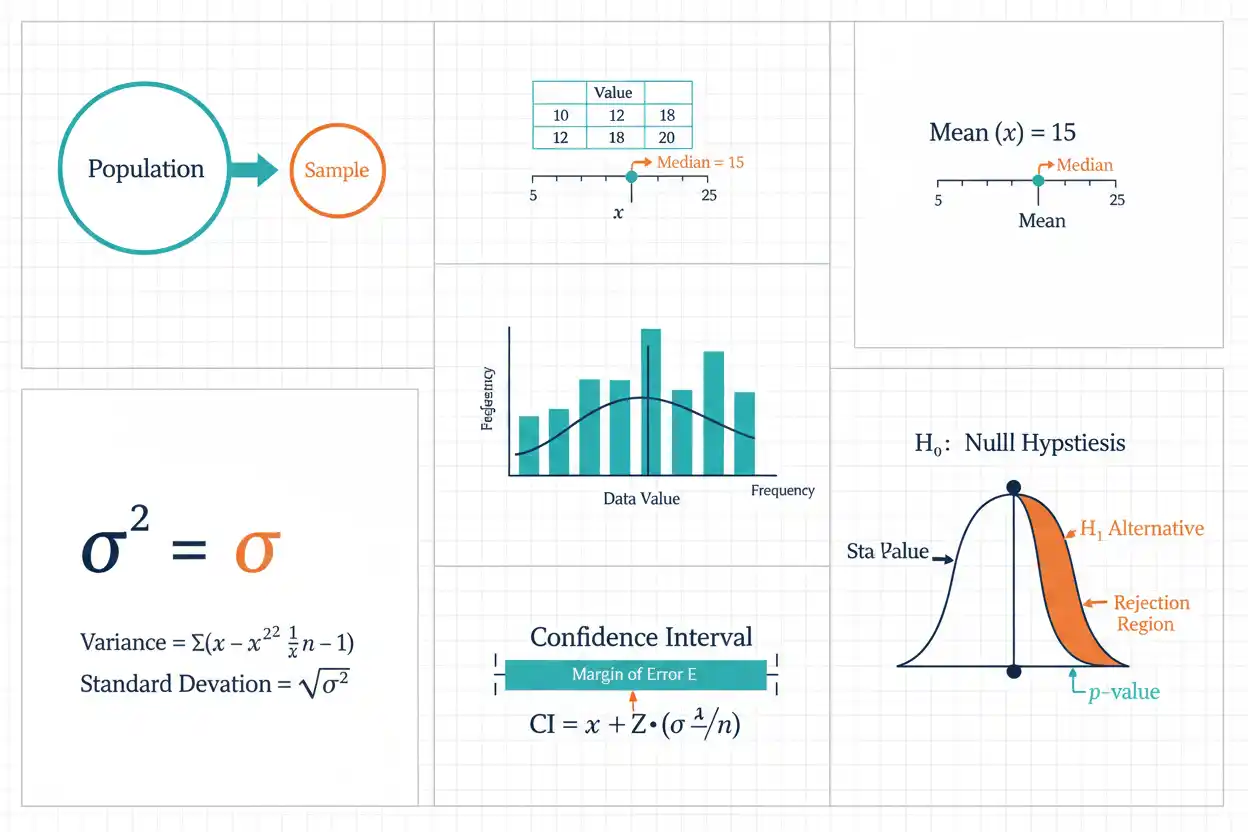
Statistics basics begin with a simple idea: data contain information about individuals, measurements, events, or processes, and statistical methods provide a structured way to summarize that information and draw carefully qualified conclusions from it. Descriptive statistics organize and summarize observed data through measures such as the mean, median, proportions, ranges, variance, standard deviation, tables, and graphs, while inferential statistics use samples to learn about larger populations through estimation, confidence intervals, hypothesis tests, and predictive models. The distinction between a population parameter and a sample statistic is fundamental because values such as the population mean μ or population proportion p are usually unknown, whereas quantities such as the sample mean x̄ or sample proportion p̂ can be calculated from observed data and used as estimates. Statistical reasoning also requires understanding variables, distributions, sampling variability, uncertainty, bias, association, and the difference between statistical significance and practical importance. Formulas provide the numerical machinery, but correct interpretation depends equally on how data were collected, whether observations are independent, how variables were measured, and whether the statistical assumptions match the problem being studied.
These statistics basics form the foundation of core statistics within the wider Statistics & Probability framework. Concepts introduced here lead naturally to specialized topics such as standard deviation, sampling distributions, statistical testing, regression, probability models, and other methods used to quantify variation and uncertainty.
What Is Statistics?
Statistics is the discipline of collecting, organizing, summarizing, analyzing, and interpreting data. It deals not only with calculations but also with the reasoning required to determine what conclusions the available evidence can support.
A statistical analysis often begins with questions such as:
- What population is being studied?
- What variables have been measured?
- How were observations selected?
- What patterns appear in the data?
- How much variability is present?
- How uncertain is an estimate?
- Does an observed difference plausibly reflect more than random sampling variation?
- Can an association be interpreted causally?
The answers determine which statistical methods are appropriate.
A correct formula applied to poorly collected or misunderstood data can still produce a misleading conclusion. Statistics therefore combines mathematics with study design and interpretation.
Descriptive Statistics
Descriptive statistics summarize the data actually observed.
Common descriptive quantities include:
Mean
Median
Mode
Minimum
Maximum
Range
Quartiles
Variance
Standard deviation
Proportions
They can also include graphical summaries such as:
Histograms
Box plots
Scatter plots
Bar charts
Descriptive statistics do not automatically generalize beyond the observed data. If a class of 30 students has an average score of 78, then:
x̄ = 78
describes that class sample.
Additional assumptions or a sampling framework are required to use the same result to estimate a broader population mean.
Inferential Statistics
Inferential statistics use sample information to learn about an unknown population quantity or process.
Examples include:
- estimating a population mean,
- estimating a population proportion,
- constructing a confidence interval,
- comparing population groups,
- testing a statistical hypothesis,
- estimating a regression coefficient.
Inference is necessary because complete population data are often unavailable.
Suppose a population contains:
1,000,000 people
but only:
n = 1,000
are sampled.
The sample may provide useful information about the population, but the result is uncertain because another random sample of 1,000 people would generally contain different individuals and produce somewhat different statistics.
Inferential statistics quantify that sampling uncertainty.
Population
A population is the complete collection of units or outcomes about which a statistical question is asked.
A population might contain:
- all registered customers of a service,
- every manufactured component in a batch,
- all students in a school system,
- every possible measurement generated by a probability process.
Population size is often represented by:
N
However, in probability models the population can be conceptual or effectively infinite rather than a finite list of physical units.
The population must be defined carefully. A statistic cannot meaningfully estimate a target population that has never been specified.
Sample
A sample is a subset of observations used to obtain information about a population.
Sample size is commonly represented by:
n
Suppose:
N = 50,000
people belong to the target population and:
n = 500
are selected for measurement.
Those 500 observations form the sample.
A larger sample size generally reduces random sampling uncertainty under an appropriate design, but increasing n does not automatically remove systematic bias. A huge nonrepresentative sample can still provide a very precise estimate of the wrong population characteristic.
Census vs Sample
A census attempts to measure every unit in the target population.
A sample measures only part of it.
If a finite population contains 1,000 employees and data are successfully collected from all 1,000, the resulting descriptive values can be treated as population quantities for that defined group.
If only 200 are measured, quantities calculated from those 200 are sample statistics.
A census removes sampling uncertainty about that particular finite population but can still contain:
- measurement error,
- missing responses,
- classification errors,
- processing mistakes.
Complete coverage does not guarantee perfect data.
Parameter
A parameter is a numerical characteristic of a population.
Common parameters include:
Population mean: μ
Population variance: σ²
Population standard deviation: σ
Population proportion: p
A parameter is treated as fixed for a defined population, although it is usually unknown.
For example, if the true average value across every unit in the target population is 75:
μ = 75
That number does not change merely because different samples are drawn.
What changes from sample to sample is the statistic used to estimate it.
Statistic
A statistic is a numerical quantity calculated from sample data.
Examples include:
Sample mean: x̄
Sample variance: s²
Sample standard deviation: s
Sample proportion: p̂
Suppose one sample gives:
x̄ = 74.6
while another gives:
x̄ = 75.8
Both can be samples from a population whose fixed mean is:
μ = 75
The variation in sample statistics across repeated samples is called sampling variability.
This distinction between parameters and statistics is one of the most important statistics basics.
Variable
A variable is a characteristic that can take different values across observations.
Examples include:
Age
Height
Number of purchases
Category membership
Response time
Test score
Variables can be numerical or categorical.
The type of variable affects which summaries and statistical methods make sense. Calculating an arithmetic mean for heights is meaningful, while calculating an arithmetic mean for labels such as red, blue, and green is not.
Categorical Variables
Categorical variables assign observations to groups or labels.
Examples include:
Product type
Region
Pass/fail status
Preferred category
A categorical variable may be nominal, where categories have no inherent numerical order, or ordinal, where categories have an ordered structure.
For example:
Low, medium, high
is ordinal.
The categories have an order, but the numerical distance between low and medium need not equal the distance between medium and high.
Categorical data are commonly summarized with counts and proportions.
Numerical Variables
Numerical variables represent quantities for which arithmetic operations are meaningful.
They can be discrete or continuous.
A discrete variable often represents counts:
0, 1, 2, 3, …
Examples include the number of calls, purchases, or defects.
A continuous variable can conceptually take any value within an interval:
2.31
2.312
2.3127
Examples include time, mass, temperature, and distance.
The distinction matters because probability models and graphical representations can differ for discrete and continuous data.
Independent and Dependent Variables
In many modeling settings, one variable is treated as a predictor and another as a response.
The predictor is often represented by:
X
and the response by:
Y
For example, a study might examine the relationship between:
X = hours studied
and:
Y = exam score.
Calling X an independent variable does not automatically mean it is statistically independent of everything else or that it causally determines Y. In regression terminology, “predictor,” “explanatory variable,” or “covariate” can often be clearer.
The causal meaning depends on study design.
Data Set
A data set is an organized collection of observations.
Suppose five observations contain values:
4, 7, 9, 10, 15
Basic descriptive analysis might calculate:
n = 5
Mean = 9
Median = 9
Minimum = 4
Maximum = 15
Range = 11
These summaries compress several observations into a few interpretable quantities.
However, no single summary describes every feature of the data, so statistical analysis often combines measures of center, spread, and shape.
Mean
The arithmetic mean is calculated by adding all observations and dividing by their number.
For a sample:
x̄ = Σxᵢ/n
Suppose:
4, 7, 9, 10, 15
Then:
x̄ = (4 + 7 + 9 + 10 + 15)/5
x̄ = 45/5
x̄ = 9
The mean uses every numerical value and is therefore sensitive to extreme observations.
It is especially useful when the arithmetic balance point of the distribution is meaningful.
Population Mean
For a finite population:
μ = Σxᵢ/N
The distinction between:
μ
and:
x̄
is conceptual rather than merely symbolic.
μ describes the actual population mean.
x̄ is calculated from a sample and commonly used to estimate μ.
If the entire population is observed, the arithmetic calculation is structurally similar, but its statistical role changes because there is no sampling uncertainty about that finite population mean.
Median
The median is the middle observation after data are sorted.
For:
2, 5, 7, 10, 30
the median is:
7
For an even number of observations:
2, 5, 7, 10
the ordinary sample median is:
(5 + 7)/2
= 6
The median depends primarily on rank and is less sensitive to extreme values than the arithmetic mean.
For skewed data, comparing the mean and median can provide useful information about asymmetry.
Mean vs Median Example
Consider:
10, 11, 12, 13, 100
The mean is:
x̄ = 146/5
x̄ = 29.2
The median is:
12
The extreme value:
100
pulls the mean strongly upward, while the median remains close to the central cluster.
Neither number is mathematically wrong.
They answer different questions.
The mean describes arithmetic balance, while the median describes the middle ranked position.
Mode
The mode is the most frequently occurring value or category.
For:
1, 2, 2, 2, 3, 4
the mode is:
2
A data set can have:
- one mode,
- several modes,
- no uniquely most frequent value.
The mode can be used with categorical data, unlike the arithmetic mean.
However, it often provides less information about numerical distribution shape than mean, median, and measures of spread.
Range
The range measures total observed span:
Range = Maximum − Minimum
For:
4, 7, 9, 10, 15
the range is:
15 − 4
= 11
The range is simple but extremely sensitive to the two most extreme observations.
If the maximum changes from:
15
to:
150
the range changes from:
11
to:
146
even though four of the five observations remain unchanged.
Variance
Variance measures average squared dispersion around the mean.
For a population:
σ² = Σ(xᵢ − μ)²/N
For a conventional sample variance estimator:
s² = Σ(xᵢ − x̄)²/(n − 1)
The distinction between population and sample variance is important because the denominators serve different purposes.
Variance is expressed in squared units. If observations are measured in meters, variance is measured in meters².
Its square root is standard deviation.
Standard Deviation
Standard deviation is:
Standard deviation = √Variance
For a population:
σ = √σ²
For a sample:
s = √s²
Because the square root returns to the original measurement units, standard deviation is often easier to interpret directly than variance.
A smaller standard deviation indicates tighter concentration around the mean, while a larger value indicates greater spread.
Its magnitude should always be interpreted relative to the data scale and distribution shape.
Worked Mean and Standard Deviation Example
Consider the sample:
4, 6, 8, 10, 12
The mean is:
x̄ = 40/5
x̄ = 8
Calculate deviations:
−4, −2, 0, 2, 4
Square them:
16, 4, 0, 4, 16
Their sum is:
40
Sample variance is:
s² = 40/(5 − 1)
s² = 10
Therefore:
s = √10
s ≈ 3.162
The sample can therefore be summarized as having mean 8 and sample standard deviation approximately 3.16.
Quartiles
Quartiles divide ordered data into broad sections.
The principal quartiles are:
Q₁ = lower quartile
Q₂ = median
Q₃ = upper quartile
Conceptually:
Q₁ ≈ 25th percentile
Q₂ = 50th percentile
Q₃ ≈ 75th percentile
Finite-sample calculation conventions differ, so small data sets can produce slightly different Q₁ and Q₃ values depending on the method.
Quartiles provide positional information rather than arithmetic averages.
Interquartile Range
The interquartile range measures the width of the middle half of a distribution:
IQR = Q₃ − Q₁
Suppose:
Q₁ = 20
and:
Q₃ = 35
Then:
IQR = 15
The IQR is less sensitive to isolated extreme observations than the overall range or standard deviation.
This makes it especially useful for skewed distributions or data containing large legitimate tail values.
Proportion
A proportion describes the fraction of observations satisfying a specified condition.
If x observations out of n have characteristic A:
p̂ = x/n
Suppose:
72
of:
120
sample observations satisfy the condition.
Then:
p̂ = 72/120
= 0.60
or:
60%
The sample proportion p̂ can be used to estimate an unknown population proportion p when the sampling process supports that inference.
Percentage vs Proportion
A proportion is commonly expressed between:
0 and 1
while a percentage expresses the same quantity on a:
0% to 100%
scale.
For example:
Proportion = 0.37
corresponds to:
Percentage = 37%
Conversion is:
Percentage = 100 × Proportion
and:
Proportion = Percentage/100
The statistical meaning is the same; only the numerical scale changes.
Frequency
Frequency is the number of times a value or category appears.
Suppose data are:
A, A, B, B, B, C
Then:
Frequency of A = 2
Frequency of B = 3
Frequency of C = 1
Relative frequency divides each count by total n.
For B:
Relative frequency = 3/6
= 0.50
Relative frequencies can be interpreted as empirical proportions.
Distribution
A distribution describes how values or probability are spread across possible outcomes.
Important features include:
- center,
- spread,
- skewness,
- tails,
- modality,
- unusual observations.
Two data sets can have identical means but very different distributions.
They can also share the same mean and standard deviation while differing in skewness or tail behavior.
Statistics basics therefore require more than reporting a single numerical summary.
Understanding distribution shape is essential for choosing appropriate methods.
Symmetric Distribution
A symmetric distribution has approximately mirrored structure around its center.
For an exactly symmetric distribution with a unique center, mean and median can coincide.
A normal distribution is a familiar example of a symmetric probability model.
Symmetry does not imply that all observations are close to the center.
A symmetric distribution can still have heavy tails or substantial variability.
The shape and spread must be considered separately.
Skewness
Skewness describes asymmetry.
A right-skewed distribution has a longer or heavier upper tail.
A left-skewed distribution has a longer or heavier lower tail.
In strongly right-skewed data, the mean is often above the median because large upper-tail values pull the arithmetic mean upward.
However, this is a tendency rather than an infallible definition of skewness.
Graphical inspection and additional distributional measures provide a more complete picture.
Outliers
An outlier is an observation that is unusually far from the main body of the data under some statistical or contextual criterion.
An outlier can be:
- a valid extreme observation,
- a measurement error,
- a recording error,
- evidence of a different subgroup,
- evidence that the assumed model is inadequate.
An unusual value should not automatically be deleted.
Its source and influence should be investigated before changing the analysis.
Statistics distinguishes statistical unusualness from confirmed data error.
Random Variable
A random variable assigns numerical values to outcomes of a random process.
A discrete random variable takes countable values, such as:
0, 1, 2, 3, …
A continuous random variable can take values throughout intervals.
Probability distributions describe how probability is allocated across these possible values.
Random variables connect descriptive statistics with probability theory and inference.
Observed data can be viewed as realizations generated by an underlying probabilistic process.
Probability
Probability measures event likelihood on a scale from:
0 to 1
An impossible event has probability:
0
A certain event has probability:
1
For an event A:
0 ≤ P(A) ≤ 1
Many statistical methods use probability to determine how much a statistic would vary under repeated samples or how unusual an observed result would be under a specified model.
Probability therefore supplies the mathematical foundation for statistical uncertainty.
Complement Rule
If Aᶜ represents the event that A does not occur:
P(Aᶜ) = 1 − P(A)
Suppose:
P(A) = 0.70
Then:
P(Aᶜ) = 0.30
This simple relationship is frequently useful when calculating probabilities such as:
at least one event
by first finding the probability that none occur.
Expected Value
Expected value is the probability-weighted mean of a random variable.
For a discrete random variable X:
E(X) = ΣxP(X=x)
Suppose X takes values:
0, 1, 2
with probabilities:
0.25, 0.50, 0.25
Then:
E(X) = 0(0.25) + 1(0.50) + 2(0.25)
= 1
Expected value describes the long-run mathematical center of the probability distribution.
It need not be an outcome that occurs in every individual trial.
Population Variability vs Sampling Variability
Population variability concerns differences among individual observations.
Sampling variability concerns differences among statistics calculated from different samples.
Suppose a population has standard deviation:
σ = 20
Samples of:
n = 100
have means whose standard error is:
σ/√n
= 20/10
= 2
Thus, individual observations vary with standard deviation 20, while sample means vary with standard deviation 2 across repeated samples.
These are different types of variation.
Sampling Distribution
A sampling distribution is the probability distribution of a statistic across hypothetical repeated samples of the same size and design.
For independent observations with population mean μ and standard deviation σ:
E(X̄) = μ
and:
SE(X̄) = σ/√n
These results are central to sampling distributions because they show why a sample mean can estimate μ with greater precision as n increases.
Statistical inference is built on the repeated-sampling behavior of estimators.
Standard Error
A standard error is the standard deviation of an estimator’s sampling distribution.
For a sample mean with known σ:
SE(X̄) = σ/√n
When σ is unknown, a common estimate is:
SÊ(X̄) = s/√n
Standard error should not be confused with standard deviation.
Standard deviation describes dispersion of observations.
Standard error describes uncertainty in an estimator.
Increasing n usually reduces standard error, but it does not automatically reduce the population standard deviation.
Central Limit Theorem
Under suitable conditions, the central limit theorem explains why standardized sample means approach a normal distribution as sample size grows.
A common form is:
Z = (X̄ − μ)/(σ/√n)
which approaches:
N(0,1)
as n becomes large under appropriate assumptions.
The theorem concerns the sampling distribution of the mean, not the distribution of raw observations.
A large sample does not make a skewed population itself normal.
It can make the distribution of certain estimators approximately normal.
Estimate
An estimate is a sample-based approximation of an unknown population parameter.
Examples include:
x̄ estimates μ
p̂ estimates p
s² estimates σ²
A point estimate provides one numerical value.
For example:
x̄ = 72.4
is a point estimate of μ.
Because another sample would generally produce a different x̄, statistical analysis often supplements point estimates with standard errors or confidence intervals.
Confidence Interval
A confidence interval provides a range generated by a statistical procedure designed to have a stated repeated-sampling coverage rate under specified assumptions.
A common approximate form is:
Estimate ± Critical value × Standard error
Suppose:
Estimate = 50
SE = 2
and an appropriate 95% critical value is:
1.96
Then:
50 ± 1.96(2)
gives:
50 ± 3.92
or:
(46.08, 53.92)
The exact critical value and standard-error formula depend on the statistical problem.
Correct Confidence-Interval Interpretation
A frequentist 95% confidence interval does not ordinarily mean:
“There is a 95% probability the fixed parameter lies inside this particular observed interval.”
Instead, the 95% refers to the long-run performance of the interval-generating procedure.
Across repeated comparable samples, approximately 95% of intervals constructed by that method contain the true parameter under the model assumptions.
This distinction is subtle but important in statistics basics because frequentist probability is attached to the random procedure rather than a fixed unknown parameter after the interval has been observed.
Hypothesis
A statistical hypothesis is a formal statement about a population parameter or probability model.
A null hypothesis is usually written:
H₀
An alternative hypothesis is:
H₁
For example:
H₀: μ = 100
H₁: μ ≠ 100
A statistical test evaluates how compatible the observed data are with H₀ according to a specified test statistic and its null sampling distribution.
It does not directly calculate whether H₀ is true with a certain probability.
Test Statistic
A test statistic standardizes the discrepancy between an observed estimate and the null hypothesis.
A generic form is:
Test statistic = (Estimate − Null value)/Standard error
For example, a one-sample t statistic is:
t = (x̄ − μ₀)/(s/√n)
The larger the absolute statistic, the farther the observed estimate lies from the null value relative to its estimated sampling uncertainty.
The reference distribution determines how unusual that statistic is under H₀.
t-Test
A t-test is used in several common mean-comparison settings when uncertainty is estimated using sample variability.
For a one-sample test:
t = (x̄ − μ₀)/(s/√n)
Under the standard one-sample t-test assumptions and H₀:
t ~ t₍ₙ₋₁₎
The t distribution has heavier tails than the standard normal distribution, particularly for small samples, because the population standard deviation is unknown and estimated from the same data.
As degrees of freedom increase, the t distribution approaches the standard normal distribution.
P-Value
A p-value measures how extreme the observed test statistic is relative to its null reference distribution.
For an upper-tailed test:
p = P(T ≥ t_obs | H₀)
A small p-value indicates that the observed statistic would be relatively unusual under the null model.
It does not mean:
P(H₀ is true) = p
and it does not measure effect size.
Statistical evidence, effect magnitude, uncertainty, and substantive importance are separate considerations.
Significance Level
A significance level is usually represented by:
α
Common values include:
0.05
0.01
A conventional decision rule is:
If p ≤ α → reject H₀
If p > α → fail to reject H₀
Failure to reject H₀ does not prove it true.
The study may have insufficient precision or power to distinguish a meaningful effect from sampling variation.
The threshold should normally be chosen before examining the result.
Type I Error
A Type I error occurs when the test rejects H₀ even though H₀ is true.
The probability of this event is controlled by the significance procedure at approximately or at most α under the appropriate null conditions.
For:
α = 0.05
the test procedure permits a 5% long-run false-rejection rate under the relevant null model.
This does not mean that exactly 5% of all statistically significant results in practice are false.
That latter probability depends on how frequently null hypotheses are true, statistical power, study selection, and other factors.
Type II Error
A Type II error occurs when H₀ is false but the test fails to reject it.
Its probability is represented by:
β
Statistical power is:
1 − β
Power depends on:
- effect size,
- sample size,
- variability,
- significance level,
- study design.
A non-significant result from a low-power study may provide weak evidence regarding whether an important effect exists.
Statistical Power
Power is the probability of rejecting H₀ when a specified alternative is true.
In general:
Larger sample size → higher power
Larger effect → higher power
Lower variability → higher power
all else equal.
Power is a study-design concept calculated before or independently of the observed p-value.
A p-value does not directly state the power of the study.
Understanding this distinction prevents several common errors in elementary inferential reasoning.
Effect Size
Effect size describes the magnitude of a difference or association.
Examples include:
Difference between means
Difference between proportions
Correlation
Standardized mean difference
A tiny effect can become statistically significant in a huge sample because standard errors become very small.
A large effect can fail to reach a conventional significance threshold in a very small sample because uncertainty is large.
Statistical significance and substantive magnitude should therefore be reported separately.
Statistical Significance vs Practical Importance
Suppose a study with an enormous sample estimates:
Difference = 0.02 units
with:
p < 0.001
The result is statistically significant.
If a difference smaller than 1 unit has no practical consequence, however, the effect may be operationally negligible.
Conversely, an estimated difference of:
10 units
with:
p = 0.08
could still be important but imprecisely measured.
Statistical significance is not a synonym for practical importance.
Correlation
Correlation measures the strength and direction of linear association between two numerical variables.
A common sample correlation coefficient is:
r
with:
−1 ≤ r ≤ 1
A positive r indicates positive linear association.
A negative r indicates negative linear association.
A value near zero indicates weak linear association, although a strong nonlinear relationship can still exist.
Correlation is symmetric: the correlation between X and Y is the same as between Y and X.
Correlation Does Not Imply Causation
A strong association does not automatically establish a causal relationship.
Suppose X and Y are highly correlated.
Possible explanations include:
- X causes Y,
- Y causes X,
- another variable affects both,
- selection creates the association,
- a shared trend produces the relationship.
Causal conclusions require appropriate design and assumptions beyond correlation.
This principle applies more broadly to regression and many observational statistical analyses.
Regression
Regression models how a response variable relates to one or more predictors.
A simple linear model can be written:
Y = β₀ + β₁X + ε
The corresponding fitted equation is:
ŷ = b₀ + b₁x
where b₁ estimates the population slope β₁.
Regression separates systematic modeled structure from residual variation.
A fitted association can be useful for prediction without necessarily having a causal interpretation.
Bias
Bias is systematic deviation of an estimator or data-collection process from the target.
For an estimator θ̂ of parameter θ:
Bias(θ̂) = E(θ̂) − θ
An unbiased estimator has:
E(θ̂) = θ
Increasing sample size reduces many forms of random sampling error, but it does not necessarily reduce systematic bias.
A huge sample drawn from the wrong population can estimate the wrong quantity extremely precisely.
Precision
Precision describes how tightly an estimator varies across repeated samples or measurements.
An estimator with a small standard error is more precise than one with a large standard error, all else equal.
Precision and accuracy are different.
A measurement process can be highly precise but systematically biased.
For example, repeated measurements:
110.0, 110.1, 109.9
are extremely consistent, but if the true value is:
100
the measurement procedure is precise yet inaccurate.
Accuracy
Accuracy describes closeness to the correct or target value.
A statistical estimate can be accurate by chance in one sample even if its estimator is noisy, while an estimator can be precise yet systematically biased.
Good statistical design aims for both:
- low systematic bias,
- adequate precision.
Sample size mainly addresses random precision under a specified design.
It cannot guarantee accuracy if the underlying sampling or measurement method is flawed.
Random Sampling
Random sampling uses a probabilistic mechanism to select units from a population.
A simple random sample gives each subset of a specified size an equal probability of selection.
Random sampling supports population inference by giving the sampling process a known probabilistic structure.
It should not be confused with random assignment.
Random sampling concerns:
who enters the sample.
Random assignment concerns:
which treatment or condition sampled units receive.
The two solve different inferential problems.
Random Assignment
Random assignment allocates experimental units to treatment conditions using a random mechanism.
Its primary purpose is to balance potential confounding variables across groups in expectation and support causal comparisons under an appropriate experiment.
A study can have:
- random sampling without random assignment,
- random assignment without random population sampling,
- both,
- neither.
Random assignment strengthens causal inference about treatment effects.
Random sampling strengthens generalization to the sampled population.
Observational Study
In an observational study, researchers observe variables without assigning the exposure or treatment through a controlled random mechanism.
Such studies can identify associations and support useful prediction.
However, causal interpretation is usually more difficult because exposed and unexposed groups can differ systematically in other ways.
Statistical adjustment can address measured confounding under assumptions, but it does not automatically reproduce the protection provided by a well-designed randomized experiment.
Experiment
An experiment deliberately applies treatments or conditions to units.
A randomized controlled experiment uses random assignment to allocate those treatments.
If implemented appropriately, randomization can make treatment groups comparable in expectation with respect to both measured and unmeasured pre-treatment characteristics.
This provides a stronger foundation for causal conclusions than an ordinary observational comparison.
Nevertheless, experiments can still face issues such as noncompliance, attrition, interference, measurement error, or poor external validity.
Confounding
A confounder is a variable associated with both an exposure and an outcome in a way that can distort the observed exposure-outcome relationship.
Suppose exercise is associated with lower disease risk, but age is associated with both exercise behavior and disease risk.
If age is ignored, part of the observed relationship may reflect age differences rather than exercise itself.
Identifying and controlling confounding requires substantive knowledge and appropriate design or modeling.
Statistical association alone cannot determine whether confounding has been eliminated.
Independence
Independence means that information about one random event or observation does not change the probability structure of another in the relevant model.
Many elementary formulas assume independent observations.
For example, if sample observations are independent with variance σ²:
Var(X̄) = σ²/n
If observations are positively correlated, this formula can underestimate uncertainty.
Repeated measurements, clustered samples, time series, and spatial data frequently violate simple independence assumptions.
The analysis must account for the actual dependence structure.
Missing Data
Missing data occur when values that should have been observed are unavailable.
Simply deleting incomplete rows can be reasonable in some settings but biased in others.
The consequence depends on why data are missing.
If missingness is related to the outcome or variables under study, the observed sample can become systematically unrepresentative.
A large remaining n does not automatically remove missing-data bias.
The mechanism generating missing values should therefore be considered in interpretation.
Measurement Error
Measurements can differ from the underlying quantity because of instrument noise, reporting mistakes, imperfect definitions, or other sources of error.
Random measurement error can increase observed variability.
Systematic measurement error can create bias.
For example, a scale that consistently adds:
2 kg
produces a systematic error.
Repeated measurements might still have a small standard deviation, demonstrating that precision and accuracy are different statistical properties.
Sampling Error
Sampling error is the difference between a sample statistic and the population parameter caused by which observations happened to be selected.
For a mean:
Sampling error = x̄ − μ
The exact sampling error is generally unknown because μ is unknown.
The standard error describes the likely scale of these sample-to-sample differences under the statistical model.
Sampling error is random.
Bias is systematic.
The two should not be treated as synonyms.
Larger Samples and Precision
For many estimators, standard error decreases approximately as:
1/√n
Suppose the standard error of a sample mean is:
4
at:
n = 25
If sample size rises to:
n = 100
the standard error becomes approximately:
2
under the same population variability and independence assumptions.
The sample size quadrupled, while standard error halved.
This square-root relationship explains why precision improves with larger samples but at diminishing returns.
Larger Samples Do Not Fix Everything
Increasing n does not automatically correct:
- biased sampling,
- invalid measurements,
- confounding,
- dependence,
- inappropriate models,
- data-entry problems.
A large sample can make a biased estimate extremely precise.
For example, if a survey excludes an important population subgroup, interviewing one million respondents from the remaining subgroup does not restore representativeness.
Statistical precision is valuable only when the target and design are appropriate.
Descriptive vs Inferential Example
Suppose 100 randomly sampled customers have:
Mean transaction value = 52
Sample standard deviation = 15
The descriptive statement is:
“The 100 observed customers had an average transaction value of 52 with sample standard deviation 15.”
An inferential statement might estimate the population mean using the sample.
The estimated standard error is:
SE = 15/√100
= 1.5
Under an appropriate large-sample procedure, a 95% interval might be approximately:
52 ± 1.96(1.5)
52 ± 2.94
giving:
(49.06, 54.94)
The first statement describes observed data; the second uses a sampling framework to make a population inference.
Parameter vs Statistic Example
Suppose the true proportion of a population with characteristic A is:
p = 0.40
A random sample of:
n = 200
contains:
86
observations with A.
Then:
p̂ = 86/200
= 0.43
Here:
p = 0.40
is the population parameter.
p̂ = 0.43
is the sample statistic.
The difference:
0.43 − 0.40 = 0.03
is sampling error for this particular hypothetical sample.
Another random sample would likely produce a different p̂.
Data Types Matter
A statistical method appropriate for one variable type may be meaningless for another.
For numerical data, it can be reasonable to calculate:
mean
variance
standard deviation.
For unordered categorical labels, the arithmetic mean is generally meaningless.
Likewise, methods designed for continuous responses may be inappropriate for binary outcomes or counts.
Correct statistical analysis begins by matching the method to the measurement scale and probability structure of the variable.
Levels of Measurement
A common classification distinguishes nominal, ordinal, interval, and ratio scales.
Nominal
Categories have no natural order.
Examples:
Color categories
Product types
Ordinal
Categories have order but not necessarily equal spacing.
Examples:
Low, medium, high
Interval
Differences are meaningful, but zero is arbitrary.
A classic example is temperature measured in Celsius.
Ratio
Differences and ratios are meaningful and zero represents absence of the measured quantity.
Examples can include length, mass, or duration.
The measurement scale influences which statistical operations are substantively interpretable.
Tables
Tables organize statistical information into rows and columns.
A frequency table can summarize categorical data:
| Category | Frequency | Proportion |
|---|---|---|
| A | 40 | 0.40 |
| B | 35 | 0.35 |
| C | 25 | 0.25 |
The proportions sum to:
1.00
or:
100%
Tables are especially useful when exact numerical values matter.
Graphs complement them by making patterns visually easier to recognize.
Histogram
A histogram groups numerical observations into intervals and displays their frequencies or densities.
It can reveal:
- center,
- spread,
- skewness,
- multiple peaks,
- gaps,
- unusual tails.
Changing bin width can alter visual appearance, so a histogram is not a completely assumption-free representation of shape.
Still, it provides information that mean and standard deviation alone cannot show.
A data set should often be graphed before complex numerical modeling begins.
Box Plot
A box plot summarizes:
Q₁
Median
Q₃
and usually displays whiskers and flagged potential outliers.
The box spans the interquartile range:
IQR = Q₃ − Q₁
Box plots are useful for comparing distributions across groups because they emphasize center and central spread.
However, they hide some details such as multimodality and exact internal density.
No single graph is sufficient for every statistical purpose.
Scatter Plot
A scatter plot displays paired numerical observations:
(xᵢ, yᵢ)
It is one of the most important tools for studying association.
A scatter plot can reveal:
- positive or negative relationships,
- curvature,
- clusters,
- changing variability,
- unusual observations.
Calculating correlation or regression without first examining the scatter plot can hide important nonlinear or subgroup patterns.
Statistical models should be checked against the structure visible in the data.
Statistic vs Estimator
An estimator is a rule or formula used to estimate a parameter.
An estimate is the numerical value produced by that estimator in one sample.
For example:
X̄
is an estimator of μ.
If the observed sample gives:
x̄ = 72.4
then:
72.4
is the estimate.
This distinction becomes useful in inference because properties such as bias and variance belong to the estimator’s repeated-sampling behavior, while the observed estimate is one realized number.
Unbiased Estimator
An estimator θ̂ is unbiased for θ if:
E(θ̂) = θ
The sample mean is unbiased for the population mean under standard sampling conditions:
E(X̄) = μ
This does not mean every sample mean equals μ.
It means that across repeated samples, the average of the sample means equals μ.
Unbiasedness concerns long-run center rather than exact accuracy in one sample.
Consistency
A consistent estimator becomes increasingly concentrated near the target parameter as sample size grows under the appropriate probabilistic conditions.
The sample mean is consistent for μ under broad assumptions.
Its variance:
σ²/n
approaches:
0
as:
n → ∞
Consistency does not mean each larger sample must be closer to μ than every smaller sample.
Random sampling can still produce occasional unusual estimates.
The property concerns asymptotic probabilistic behavior.
Statistical Model
A statistical model specifies assumptions about how observed data are generated.
A simple model might state:
Y = μ + ε
where ε represents random variation around μ.
A regression model might state:
Y = β₀ + β₁X + ε
A probability distribution might specify the form of ε or Y.
Models simplify reality so that quantities can be estimated and uncertainty calculated.
The usefulness of a statistical result therefore depends partly on whether the model captures the important structure of the data.
Assumptions Matter
Common statistical assumptions can involve:
- independence,
- random sampling,
- distribution shape,
- equal variance,
- linearity,
- correct model specification.
Not every statistical method requires all of these assumptions.
For example, normality is relevant in some small-sample procedures but not a universal requirement for every calculation.
The correct approach is to identify the assumptions of the specific method being used rather than apply a generic checklist to every analysis.
Association vs Causation
Statistics can quantify an association without establishing its causal origin.
Suppose two variables have correlation:
r = 0.80
This indicates strong positive linear association in the observed sample.
It does not by itself tell us whether:
X causes Y
Y causes X
or:
another factor influences both.
Causal conclusions require additional assumptions and usually stronger study design.
This distinction remains essential no matter how large or statistically significant the association becomes.
Statistical vs Scientific Uncertainty
A statistical confidence interval can quantify uncertainty arising from a defined sampling model.
It does not automatically capture every uncertainty in a real study.
Other uncertainty can come from:
- measurement definitions,
- missing data,
- model selection,
- data processing,
- external validity,
- confounding,
- changing conditions.
A very narrow statistical confidence interval should therefore not be mistaken for complete certainty about the broader real-world question.
Statistical uncertainty is one component of evidential uncertainty.
Common Statistics Basics Mistakes
A common mistake is confusing a population parameter with a sample statistic. The population mean μ is fixed for the defined population, while x̄ changes from sample to sample.
Another error is assuming that a large sample automatically removes bias. Larger n generally reduces random sampling variability but cannot correct a systematically unrepresentative sampling process.
Another frequent mistake is confusing standard deviation with standard error. Standard deviation describes observation-level variability, while standard error describes estimator variability across repeated samples.
Analysts also sometimes interpret correlation or regression as proof of causation, even when the data are observational.
Another mistake is saying that a p-value is the probability that the null hypothesis is true. It is instead a probability calculated under the null model concerning results at least as extreme as the observed test statistic.
A non-significant result should not be interpreted as proof of no effect, just as a statistically significant result should not automatically be interpreted as practically important.
Finally, summary statistics should not replace examination of the underlying distribution because very different data structures can share the same mean, variance, or correlation.
How to Analyze Basic Statistics Step by Step
Begin by defining the population, observational unit, variables, and research question. Determine whether each variable is categorical or numerical and whether the goal is descriptive, inferential, predictive, or causal, because these distinctions affect every later choice.
Next examine the data for missing values, impossible entries, unusual observations, and measurement inconsistencies. Summarize numerical variables using an appropriate combination of center and spread, and use frequency or proportion summaries for categorical variables. Graph the distributions and important relationships so that skewness, clusters, curvature, or unusual observations are not hidden by a single summary statistic.
If inference is required, identify how the sample was obtained, determine the appropriate sampling distribution or statistical model, calculate standard errors or confidence intervals, and check the assumptions relevant to the method. Interpret the results in terms of effect magnitude and uncertainty rather than relying on a threshold alone.
Full Statistics Basics Example
Suppose a random sample of eight observations is:
6, 7, 8, 8, 9, 10, 10, 14
The sample size is:
n = 8
Calculate the Mean
x̄ = (6 + 7 + 8 + 8 + 9 + 10 + 10 + 14)/8
x̄ = 72/8
x̄ = 9
Calculate the Median
The middle observations are:
8 and 9
Therefore:
Median = (8 + 9)/2
= 8.5
Calculate the Range
Range = 14 − 6
= 8
Calculate the Sample Variance
Deviations from the mean are:
−3, −2, −1, −1, 0, 1, 1, 5
Squared deviations are:
9, 4, 1, 1, 0, 1, 1, 25
Their sum is:
42
Therefore:
s² = 42/(8 − 1)
s² = 6
Calculate the Sample Standard Deviation
s = √6
s ≈ 2.449
Thus the data have:
Mean = 9
Median = 8.5
Sample variance = 6
Sample standard deviation ≈ 2.45
The maximum value of 14 creates some upper-tail extension, reflected in the mean being slightly above the median.
Inferring a Population Mean From the Example
If those eight observations were an appropriate independent sample from a larger population, the estimated standard error of the mean would be:
SÊ(X̄) = s/√n
= 2.449/√8
≈ 2.449/2.828
≈ 0.866
The point estimate of μ is:
x̄ = 9
but the population mean is not known exactly.
The standard error quantifies how sample means of this size would vary under the inferential model.
Because n is small and σ is unknown, a t-based procedure rather than an ordinary z procedure would typically be used for classical normal-theory inference about μ.
Why the Example Does Not Prove the Population Mean
Even though:
x̄ = 9
we should not conclude:
μ = 9
with certainty.
Another random sample could produce:
x̄ = 8.4
or:
x̄ = 9.7
or another value.
The sample mean is evidence about μ, not direct observation of μ.
This distinction between an observed statistic and an unknown parameter is the core problem that inferential statistics is designed to address.
Descriptive Statistics Checklist
For a basic numerical data set, useful questions include:
What is the sample size?
What is the mean?
What is the median?
What is the spread?
Are there extreme observations?
Is the distribution symmetric or skewed?
Are there clusters or gaps?
For categorical data, ask:
What categories occur?
How frequent is each category?
What proportion belongs to each group?
These questions provide a foundation before more advanced inference or modeling begins.
Inferential Statistics Checklist
When generalizing from a sample, ask:
What is the target population?
How was the sample selected?
Are observations independent or appropriately modeled?
What parameter is being estimated?
What is the estimator’s standard error?
What assumptions determine its sampling distribution?
How large is the effect?
How uncertain is the estimate?
Are conclusions being interpreted beyond what the design supports?
These questions are more important than simply obtaining a small p-value or narrow interval.
How to Report Basic Statistics
A clear statistical summary should identify the sample, the variables, the center and spread, and any important inferential quantities.
For approximately symmetric numerical data, a report might state:
“The sample contained n = 100 observations, with mean 52.3 and sample standard deviation 8.4.”
For skewed data, it may be more useful to report:
“The median was 48, with Q₁ = 35 and Q₃ = 66.”
When inference is included, state the estimate and uncertainty:
“The estimated mean was 52.3 with a 95% confidence interval from 50.6 to 54.0.”
The appropriate summary should reflect the data structure rather than forcing every variable into the same reporting template.
Frequently Asked Questions About Statistics Basics
What is statistics?
Statistics is the discipline of collecting, organizing, analyzing, and interpreting data while quantifying variation and uncertainty.
What are the two main branches of statistics?
They are:
Descriptive statistics
and:
Inferential statistics.
What are descriptive statistics?
They summarize the observations actually collected using quantities such as mean, median, proportions, variance, standard deviation, and graphical displays.
What are inferential statistics?
They use sample information and probability models to estimate or test statements about larger populations.
What is a population?
A population is the complete set of units or outcomes to which a statistical question refers.
What is a sample?
A sample is a subset of observations selected from or representing a target population.
What is a parameter?
A parameter is a numerical characteristic of a population, such as μ, σ², σ, or p.
What is a statistic?
A statistic is a numerical quantity calculated from sample observations, such as x̄, s², s, or p̂.
What is the sample mean formula?
x̄ = Σxᵢ/n
What is the population mean formula?
μ = Σxᵢ/N
for a finite population.
What is variance?
Variance measures squared dispersion around the mean.
What is the sample variance formula?
s² = Σ(xᵢ − x̄)²/(n − 1)
What is standard deviation?
Standard deviation is the square root of variance and measures dispersion in the original units of the data.
What is the difference between standard deviation and standard error?
Standard deviation measures variability among observations. Standard error measures variability of an estimator across repeated samples.
What is the median?
The median is the middle ranked value of an ordered data set.
What is the mode?
The mode is the most frequently occurring value or category.
What is the range?
Range = Maximum − Minimum
What is the interquartile range?
IQR = Q₃ − Q₁
It describes the width of the middle 50% of the distribution.
What is a proportion?
A sample proportion is:
p̂ = x/n
where x is the number of observations satisfying the event of interest.
What is a variable?
A variable is a characteristic that can take different values across observations.
What is the difference between categorical and numerical data?
Categorical variables represent labels or groups, while numerical variables represent quantities for which arithmetic operations can be meaningful.
What is a sampling distribution?
It is the distribution of a statistic across repeated samples generated under the same sampling procedure.
What is the standard error of the mean?
For independent observations with known population standard deviation:
SE(X̄) = σ/√n
Why does sample size matter?
Larger samples generally reduce sampling variability and improve estimator precision under an appropriate statistical design.
Does a large sample guarantee accurate results?
No. A large sample does not automatically fix bias, poor measurements, confounding, dependence, or an inappropriate model.
What is the central limit theorem?
Under suitable conditions, it explains why standardized sample means become approximately normally distributed as sample size grows.
Does the central limit theorem make the raw data normal?
No. It concerns the sampling distribution of certain statistics, not the underlying raw-data distribution.
What is a confidence interval?
It is an interval generated by a procedure designed to achieve a specified long-run coverage rate under statistical assumptions.
What is a hypothesis test?
It is a procedure that evaluates how compatible observed data are with a specified null hypothesis using a test statistic and reference distribution.
What is a p-value?
A p-value is a tail probability calculated under the null hypothesis for a test statistic at least as extreme as the observed one.
Does p = 0.05 mean the null hypothesis has a 5% chance of being true?
No.
What is statistical power?
Power is the probability of rejecting the null hypothesis when a specified alternative is true.
What is a Type I error?
It occurs when a true null hypothesis is rejected.
What is a Type II error?
It occurs when a false null hypothesis is not rejected.
Does statistical significance mean practical importance?
No. A statistically significant effect can be too small to matter practically.
Does correlation prove causation?
No. Correlation measures association, not causal direction.
What is bias?
Bias is systematic deviation of an estimator or data-collection process from the target value.
What is precision?
Precision refers to how tightly repeated estimates or measurements cluster.
What is sampling error?
Sampling error is the random difference between a sample statistic and its corresponding population parameter caused by the particular sample selected.
What is random sampling?
It is a probabilistic procedure for selecting observations from a population.
What is random assignment?
It is a probabilistic procedure for assigning experimental units to treatment conditions and serves a different purpose from random sampling.
What is the most important principle in statistics basics?
Define the population and variables clearly, understand how the data were collected, distinguish sample statistics from population parameters, quantify both center and variation, and interpret statistical uncertainty within the limits of the study design rather than relying on formulas alone.




