

Sampling Distributions: Definition, Formula & Example

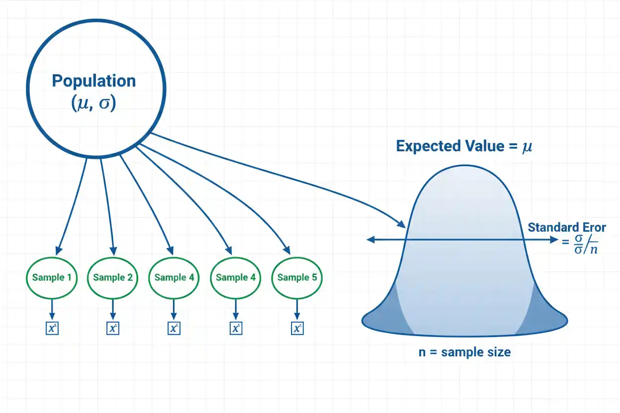
Sampling distributions describe how a statistic changes across repeated random samples drawn from the same population under the same sampling procedure. Instead of examining the distribution of individual observations, sampling distributions focus on quantities calculated from samples—such as the sample mean, sample proportion, variance, regression slope, or difference between two means—and ask how those statistics would vary if the sampling process were repeated many times. This distinction is fundamental because statistical inference depends on uncertainty in an estimator rather than simply variability among individual observations. For example, a population may have a standard deviation of 12 units, yet the sampling distribution of the mean from samples of 36 observations has a standard deviation of only 2 units, showing that sample averages vary much less than individual measurements. That standard deviation of a sampling distribution is called the standard error. As sample size increases, sampling distributions of many common estimators become more concentrated around their population targets, while the central limit theorem explains why the sampling distribution of a properly standardized sample mean often becomes approximately normal under suitable conditions even when the population itself is not normal. Understanding sampling distributions therefore provides the mathematical bridge from observed sample statistics to confidence intervals, hypothesis tests, margins of error, and assessments of estimator precision.
Sampling distributions are a central part of core statistics and the broader Statistics & Probability framework. The distinction between population parameters and sample statistics begins with statistics basics, while the width of sampling distributions depends strongly on sample size and population variability.
What Are Sampling Distributions?
A sampling distribution is the probability distribution of a statistic over all possible samples of a specified size generated under a defined sampling process.
Suppose a population has unknown mean:
μ
and repeated random samples of size:
n
are drawn. From each sample, calculate the sample mean:
x̄
One sample might produce:
x̄ = 48.7
another:
x̄ = 50.4
another:
x̄ = 49.8
and another:
x̄ = 51.1
If the sampling process were repeated an enormous number of times and every resulting x̄ were recorded, those means would form the sampling distribution of the sample mean.
The same idea applies to other statistics. Repeated samples produce different sample proportions, variances, medians, regression slopes, and other estimates, so each statistic has its own sampling distribution determined by the population, sample size, sampling design, and estimator.
Population Distribution vs Sample Distribution vs Sampling Distribution
These three concepts are frequently confused, yet they describe different objects. The population distribution describes individual values throughout the full population. A sample distribution describes the individual observations contained in one realized sample. A sampling distribution describes a statistic calculated from many hypothetical repeated samples.
Suppose individual population values have:
Mean = 50
Standard deviation = 12
A particular sample of 36 observations may contain values ranging widely around 50. Its own sample distribution describes those 36 raw observations.
Now imagine repeatedly drawing samples of 36 and calculating a mean from each one. The resulting collection of sample means forms a new distribution—the sampling distribution of x̄.
Its center is:
μ = 50
but its spread is only:
12/√36 = 2
under independent sampling.
The population and sampling distributions therefore have the same mean in this case but very different variability.
What Is a Statistic?
A statistic is a numerical quantity calculated from sample data.
Examples include:
Sample mean: x̄
Sample proportion: p̂
Sample variance: s²
Sample standard deviation: s
Regression slope: b₁
A parameter is the corresponding fixed population quantity, such as:
Population mean: μ
Population proportion: p
Population variance: σ²
Population regression slope: β₁
A statistic varies from sample to sample. A population parameter is treated as fixed for the target population.
Sampling distributions describe that sample-to-sample variability of statistics.
Why Statistics Vary Across Samples
Consider a population containing many different values. One random sample can, by chance, include slightly more high observations, while another contains more low observations. Their sample means will therefore differ even when both samples were collected correctly from the same population.
This variation is called:
sampling variability
It does not automatically indicate a measurement problem or biased procedure. Random sampling itself creates variation because different samples contain different observations.
Sampling distributions quantify that natural fluctuation.
If an estimator has a narrow sampling distribution, repeated samples tend to give similar estimates. If the sampling distribution is wide, estimates vary considerably from sample to sample.
Sampling Distribution of the Sample Mean
Suppose:
X₁, X₂, …, Xₙ
are independent observations from a population with:
E(Xᵢ) = μ
and:
Var(Xᵢ) = σ²
The sample mean is:
X̄ = (X₁ + X₂ + … + Xₙ)/n
Its expected value is:
E(X̄) = μ
Its variance is:
Var(X̄) = σ²/n
and its standard deviation is:
SD(X̄) = σ/√n
The standard deviation of a statistic’s sampling distribution is called its standard error, so:
SE(X̄) = σ/√n
This formula shows why averaging several independent observations produces a more stable quantity than relying on one observation.
Why the Mean of X̄ Equals μ
Starting with:
X̄ = (X₁ + X₂ + … + Xₙ)/n
take the expectation:
E(X̄) = E[(X₁ + X₂ + … + Xₙ)/n]
Using linearity of expectation:
E(X̄) = [E(X₁) + E(X₂) + … + E(Xₙ)]/n
If every observation has population mean μ:
E(X̄) = (nμ)/n
Therefore:
E(X̄) = μ
The sample mean is therefore an unbiased estimator of the population mean under the usual sampling setup.
Across repeated samples, its average value equals the population mean.
Why the Variance of X̄ Is σ²/n
For independent observations:
Var(X₁ + … + Xₙ) = Var(X₁) + … + Var(Xₙ)
Since every observation has variance σ²:
Var(X₁ + … + Xₙ) = nσ²
Because:
X̄ = (1/n)(X₁ + … + Xₙ)
variance scales by the square of the constant:
Var(X̄) = (1/n²)(nσ²)
Therefore:
Var(X̄) = σ²/n
Taking the square root gives:
SE(X̄) = σ/√n
This derivation depends on independence or an equivalent covariance structure. If observations are correlated, covariance terms can change the variance substantially.
Sampling Distribution Example
Suppose a population has:
μ = 50
σ = 12
and samples contain:
n = 36
independent observations.
The sampling distribution of the sample mean has:
E(X̄) = 50
and:
SE(X̄) = 12/√36
= 12/6
= 2
Therefore, the sample means are centered at:
50
with standard error:
2
Even though individual population observations have standard deviation 12, sample means based on 36 observations vary much less.
This is the central advantage of averaging independent information.
Exact Normal Sampling Distribution
If the population itself is normally distributed:
Xᵢ ~ N(μ, σ²)
then the sample mean is exactly normal for every positive integer n:
X̄ ~ N(μ, σ²/n)
For the previous example, if the population is normal:
X̄ ~ N(50, 4)
because:
σ²/n = 144/36
= 4
and the standard error is:
√4 = 2
No large-sample approximation is required in this case.
Normality of the sampling distribution follows exactly from the fact that linear combinations of independent normal random variables are normal.
Probability Example Using a Sampling Distribution
Continue with:
μ = 50
σ = 12
n = 36
and assume the sampling distribution of X̄ is normal.
Find:
P(X̄ > 54)
The standard error is:
SE = 2
Standardize:
z = (54 − 50)/2
z = 2
Therefore:
P(X̄ > 54) = P(Z > 2)
Using the standard normal distribution:
P(Z > 2) ≈ 0.0228
Thus:
P(X̄ > 54) ≈ 2.28%
Even though individual observations greater than 54 may be common in a population with standard deviation 12, a sample mean of 36 observations exceeding 54 is much less common because averages have substantially smaller variability.
Probability Between Two Sample Means
Using the same population and sample size, find:
P(48 ≤ X̄ ≤ 52)
The standard error remains:
2
For the lower boundary:
z = (48 − 50)/2
z = −1
For the upper boundary:
z = (52 − 50)/2
z = 1
Therefore:
P(48 ≤ X̄ ≤ 52) = P(−1 ≤ Z ≤ 1)
For the standard normal distribution:
P(−1 ≤ Z ≤ 1) ≈ 0.6827
Thus, approximately:
68.27%
of repeated sample means would lie between 48 and 52 under this model.
Standard Error
A standard error is the standard deviation of a sampling distribution.
For the sample mean:
SE(X̄) = σ/√n
when σ is known.
When σ is unknown, the estimated standard error is usually:
SÊ(X̄) = s/√n
where s is the sample standard deviation.
The standard deviation and standard error describe different kinds of variation. Standard deviation describes how individual observations vary, while standard error describes how an estimator varies across repeated samples.
Confusing these quantities can greatly misrepresent uncertainty.
Standard Deviation vs Standard Error
Suppose a population has:
σ = 20
and:
n = 100
Then individual observations have population standard deviation:
20
but the sample mean has standard error:
20/√100
= 2
Increasing n does not make the population observations less variable. Their standard deviation remains 20.
It makes the sample mean more stable across repeated samples.
This distinction is one of the most important ideas behind sampling distributions.
Effect of Sample Size
The standard error of a sample mean follows:
SE = σ/√n
Suppose:
σ = 20
Then:
| Sample size n | SE of X̄ |
|---|---|
| 25 | 4 |
| 100 | 2 |
| 400 | 1 |
| 1,600 | 0.5 |
Each fourfold increase in sample size halves the standard error.
This square-root relationship means larger samples increase precision, but with diminishing returns. Doubling n reduces standard error only by a factor of:
1/√2 ≈ 0.707
rather than cutting it in half.
Central Limit Theorem
The central limit theorem explains why sampling distributions of sums and means often become approximately normal even when individual population observations are not normally distributed.
In a common independent-identically-distributed version, if X₁,…,Xₙ have finite mean μ and finite positive variance σ², then:
(X̄ − μ)/(σ/√n)
approaches the standard normal distribution as:
n → ∞
Thus:
X̄ ≈ N(μ, σ²/n)
for sufficiently large n under suitable conditions.
The theorem concerns the sampling distribution of the standardized mean, not the raw population distribution.
The Central Limit Theorem Does Not Make Data Normal
Suppose individual observations follow a strongly right-skewed distribution.
Increasing the sample size from:
20
to:
2,000
does not cause the raw observations themselves to become normal. The population can remain strongly skewed indefinitely.
What becomes increasingly normal under central-limit conditions is the distribution of:
X̄
across hypothetical repeated samples.
This distinction prevents a common mistake:
Large sample → raw data are normal
is false.
The correct idea is:
Large sample → certain standardized estimators may have approximately normal sampling distributions.
How Large Must n Be?
There is no universal sample-size threshold that guarantees an adequate normal approximation.
A nearly symmetric population may produce a reasonably normal sampling distribution of the mean with a modest n. A highly skewed or heavy-tailed population can require a considerably larger sample, while a population with infinite variance may violate the usual finite-variance central-limit framework entirely.
The required n also depends on the level of accuracy needed. Approximation near the center of a distribution can become adequate sooner than approximation in very extreme tails.
Rules such as:
n ≥ 30
are therefore heuristics, not universal mathematical guarantees.
Sampling Distribution of a Sample Proportion
Suppose each independent observation is binary:
Xᵢ = 1 if event occurs
Xᵢ = 0 otherwise
with:
P(Xᵢ = 1) = p
The sample proportion is:
p̂ = X/n
where X is the number of successes.
Its expected value is:
E(p̂) = p
and variance is:
Var(p̂) = p(1 − p)/n
Therefore:
SE(p̂) = √[p(1 − p)/n]
The sample proportion is an unbiased estimator of the population proportion under independent Bernoulli sampling.
Sample Proportion Example
Suppose:
p = 0.40
and:
n = 100
Then:
E(p̂) = 0.40
and:
SE(p̂) = √[(0.40)(0.60)/100]
= √0.0024
≈ 0.0490
Therefore, repeated sample proportions are centered at:
0.40
with standard error approximately:
0.049
or about:
4.9 percentage points.
The actual sampling distribution is discrete because p̂ can take only values:
0, 0.01, 0.02, …, 1.00
for n = 100, although a normal approximation can often be useful when the binomial conditions support it.
Normal Approximation for a Sample Proportion
Because:
np̂
arises from a binomial count, the sampling distribution of p̂ can often be approximated by a normal distribution when expected successes and failures are sufficiently numerous.
A common practical check examines:
np
and:
n(1 − p)
The exact adequacy required depends on the application rather than one universal threshold.
When the approximation is suitable:
p̂ ≈ N[p, p(1 − p)/n]
This allows standard-normal probability calculations and provides the basis for many large-sample procedures involving proportions.
Sampling Distribution of the Difference Between Means
Suppose two independent samples have:
X̄₁ with mean μ₁ and variance σ₁²/n₁
and:
X̄₂ with mean μ₂ and variance σ₂²/n₂
Then:
E(X̄₁ − X̄₂) = μ₁ − μ₂
and, under independence:
Var(X̄₁ − X̄₂) = σ₁²/n₁ + σ₂²/n₂
Therefore:
SE(X̄₁ − X̄₂) = √(σ₁²/n₁ + σ₂²/n₂)
This sampling distribution is central to statistical comparisons between two population means.
Difference Between Means Example
Suppose:
μ₁ = 70
σ₁ = 10
n₁ = 100
and:
μ₂ = 65
σ₂ = 8
n₂ = 64
The expected difference is:
E(X̄₁ − X̄₂) = 70 − 65
= 5
The standard error is:
SE = √(10²/100 + 8²/64)
= √(1 + 1)
= √2
≈ 1.414
Thus, repeated differences between the two sample means are centered at 5 with standard error approximately 1.414 under the stated independent-sampling model.
If the population distributions are normal, the difference is exactly normal. Under broader conditions, a suitable large-sample normal approximation can follow from central-limit arguments.
Sampling Distribution of a Difference Between Proportions
For two independent population proportions p₁ and p₂:
E(p̂₁ − p̂₂) = p₁ − p₂
and:
Var(p̂₁ − p̂₂) = p₁(1 − p₁)/n₁ + p₂(1 − p₂)/n₂
Therefore:
SE(p̂₁ − p̂₂) = √[p₁(1−p₁)/n₁ + p₂(1−p₂)/n₂]
This distribution provides the foundation for confidence intervals comparing two proportions.
For hypothesis testing under a null hypothesis such as:
p₁ = p₂
the estimated standard error can use a pooled proportion depending on the specific test. The confidence-interval and hypothesis-test formulas should therefore not be assumed identical without checking the procedure.
Sampling With Replacement
If observations are sampled independently with replacement from a population, each draw has the same distribution and one observation does not alter the probabilities for future draws.
This structure makes variance calculations such as:
Var(X̄) = σ²/n
particularly straightforward.
Many theoretical results use independent sampling as their basic framework.
Real-world designs can deviate from this ideal through finite-population sampling, clustering, time dependence, repeated measurements, or other structures.
Those deviations can change sampling distributions even when the raw sample size is unchanged.
Sampling Without Replacement
Suppose n units are sampled without replacement from a finite population of size N.
The observations are then negatively dependent because once a unit is selected, it cannot be selected again.
For a simple random sample without replacement, the standard error of the mean can include a finite population correction:
SE(X̄) = (σ/√n)√[(N − n)/(N − 1)]
The factor:
√[(N − n)/(N − 1)]
is smaller than 1 when n > 1.
As the sampled fraction becomes substantial, the sampling distribution narrows because observing a large fraction of the population leaves less uncertainty about its mean.
Finite Population Example
Suppose:
N = 1,000
n = 400
and the finite population standard deviation is:
σ = 20
Ignoring finite population correction gives:
SE = 20/√400
= 1
The correction factor is:
√[(1000 − 400)/(1000 − 1)]
= √(600/999)
≈ 0.775
Therefore:
SE ≈ 0.775
Sampling 40% of the finite population without replacement provides more information than 400 independent draws from an effectively infinite population.
Bias
An estimator is unbiased for a parameter θ if:
E(θ̂) = θ
The sample mean satisfies:
E(X̄) = μ
so it is unbiased for μ.
A biased estimator satisfies:
E(θ̂) ≠ θ
Its sampling distribution is centered away from the target parameter.
Bias concerns the center of a sampling distribution.
Precision concerns its spread.
An estimator can be unbiased but highly variable, or biased but tightly concentrated.
These are separate statistical properties.
Bias Example
Suppose an estimator T has sampling distribution with:
E(T) = 102
when the true parameter is:
θ = 100
Then:
Bias(T) = E(T) − θ
= 102 − 100
= 2
The estimator is systematically high by two units on average across repeated samples.
Increasing sample size can sometimes reduce an estimator’s bias, but it does not universally remove systematic bias. If the underlying sampling procedure consistently excludes part of the target population, a huge sample can remain biased.
Variance of an Estimator
The variance of an estimator describes how widely its values fluctuate across repeated samples:
Var(θ̂) = E[(θ̂ − Eθ̂)²]
A smaller estimator variance indicates greater precision.
For the sample mean under independent sampling:
Var(X̄) = σ²/n
so precision improves as n grows.
Two estimators can target the same population parameter but have different sampling variances. Statistical efficiency concerns how much information an estimator extracts relative to competing estimators under a specified model.
Mean Squared Error
Mean squared error combines bias and variance:
MSE(θ̂) = E[(θ̂ − θ)²]
It can be decomposed as:
MSE(θ̂) = Var(θ̂) + [Bias(θ̂)]²
This illustrates an important tradeoff. An estimator with a small amount of bias can sometimes have lower total mean squared error than an unbiased estimator with very high variance.
Sampling distributions make this comparison possible because both bias and variance are properties of an estimator’s repeated-sampling behavior.
Consistency
An estimator is consistent if it converges toward the true parameter as sample size grows under the relevant probabilistic definition.
Informally:
larger samples make the estimator increasingly concentrated near the target.
The sample mean is consistent for μ under broad conditions because its variance:
σ²/n
approaches zero as:
n → ∞
while its expected value remains μ.
Consistency is an asymptotic property. It does not mean every larger sample must produce an estimate closer to the truth than every smaller sample.
Random variation can still make one individual larger sample less accurate than a particular smaller sample.
Standardized Sampling Distributions
A statistic is often standardized by subtracting its expected value and dividing by its standard error.
For a sample mean with known σ:
Z = (X̄ − μ)/(σ/√n)
If the underlying population is normal:
Z ~ N(0,1)
exactly.
Under central-limit conditions:
Z ≈ N(0,1)
for sufficiently large n.
Standardization converts the estimator into a common reference scale, making probability calculations and inferential procedures possible across many measurement units.
Unknown Population Standard Deviation
In practice, σ is often unknown.
Replacing σ by the sample standard deviation s gives:
(X̄ − μ)/(s/√n)
If the observations are independent and come from a normal population, this statistic follows Student’s t distribution:
T ~ t₍ₙ₋₁₎
The use of s introduces additional uncertainty compared with knowing σ exactly.
That uncertainty produces heavier tails in the t distribution, particularly for small n.
As n grows, the t distribution approaches the standard normal distribution.
Sampling Distribution of the Sample Variance
The sampling distribution of the sample variance has a particularly important exact form under normal sampling.
If:
X₁,…,Xₙ ~ independent N(μ,σ²)
and:
S² = Σ(Xᵢ − X̄)²/(n − 1)
then:
(n − 1)S²/σ² ~ χ²₍ₙ₋₁₎
This chi-square sampling distribution forms the basis of classical confidence intervals and hypothesis tests for a normal population variance.
Unlike the sampling distribution of the mean, the variance distribution is generally right-skewed, especially when n is small.
It becomes relatively more concentrated as sample size increases.
Why Sample Variance Uses n − 1
The sample variance:
S² = Σ(Xᵢ − X̄)²/(n − 1)
uses:
n − 1
rather than n so that:
E(S²) = σ²
under independent identically distributed sampling with finite variance.
Using the estimated sample mean costs one degree of freedom because the deviations satisfy:
Σ(Xᵢ − X̄) = 0
Only n − 1 deviations can vary freely after the sample mean is fixed.
The resulting estimator S² is unbiased for population variance.
Sampling Distribution of a Regression Slope
A fitted regression line also produces sample-dependent coefficients.
If repeated samples were collected, each would generally produce a different:
b₁
for the regression slope.
Under the classical simple linear regression model and conditioning on the observed predictor values:
E(b₁) = β₁
and:
Var(b₁) = σ²/Sxx
where:
Sxx = Σ(xᵢ − x̄)²
Under normally distributed regression errors:
b₁
has an exact normal sampling distribution before σ is estimated, and:
(b₁ − β₁)/SE(b₁)
follows a t distribution with:
n − 2
degrees of freedom when σ is replaced by the residual estimate.
This illustrates that regression inference is fundamentally another application of sampling distributions.
Sampling Distribution of the Median
The sample median also changes from sample to sample.
Its sampling distribution can be more complicated than that of the mean because it depends on order statistics and the population density near the median.
Under suitable smoothness conditions and large n, a sample quantile has an approximately normal sampling distribution.
For a continuous population with median m and density f(m) > 0, the sample median has approximate variance:
Var(Median) ≈ 1/[4n f(m)²]
This formula shows that median precision depends not only on n but also on how densely population values are concentrated near the median.
Sampling Distributions of Quartiles
Sample quartiles likewise vary across repeated samples.
One random sample may produce:
Q₁ = 20
while another from the same population gives:
Q₁ = 22
or:
Q₁ = 19.5
The variability depends on sample size, the quartile estimator, and the population density near the target quantile.
Quartiles in small samples can be especially variable because only a few ordered observations determine their locations. Different finite-sample quartile conventions can introduce additional numerical differences that are separate from random sampling variability.
Sampling Distribution and Confidence Intervals
A confidence interval uses knowledge of an estimator’s sampling distribution to construct a range with specified repeated-sampling coverage.
For a mean with known σ and an appropriate normal sampling distribution:
X̄ ~ N(μ, σ²/n)
standardization gives:
Z = (X̄ − μ)/(σ/√n)
Approximately 95% of standard normal values lie between:
−1.96 and 1.96
Therefore:
P[−1.96 ≤ (X̄ − μ)/(σ/√n) ≤ 1.96] = 0.95
Rearranging yields the familiar interval procedure:
X̄ ± 1.96σ/√n
The confidence level comes directly from the sampling distribution.
Sampling Distribution and Hypothesis Tests
Hypothesis testing also relies on sampling distributions.
Suppose:
H₀: μ = μ₀
Under the null hypothesis, determine the sampling distribution of the test statistic.
For a known-σ mean test:
Z = (X̄ − μ₀)/(σ/√n)
Under H₀ and the required assumptions:
Z ~ N(0,1)
A p-value is then calculated from the tail probability of this null sampling distribution.
The observed statistic is judged according to how unusual it would be if repeated samples truly came from the null model.
Without a reference sampling distribution, there is no principled basis for the standard p-value calculation.
Sampling Distribution and Margin of Error
A margin of error is typically:
Critical value × Standard error
For a 95% large-sample mean interval:
E = 1.96σ/√n
The critical value comes from the shape of the standardized sampling distribution, while the standard error determines its scale.
Increasing sample size decreases the standard error, narrowing the margin of error.
Increasing confidence raises the critical value, widening the margin.
The structure of sampling distributions therefore explains the tradeoff among confidence, precision, sample size, and variability.
Sampling Error
Sampling error is the difference between a sample statistic and the corresponding population parameter caused by the particular observations selected.
For a mean:
Sampling error = X̄ − μ
This quantity is usually unknown in a real study because μ itself is unknown.
The sampling distribution describes the possible behavior of this error across repeated samples.
Standard error does not equal the actual sampling error from one particular sample. It describes the typical scale of sampling errors under the model.
Standard Error Is Not an Error Count
The phrase standard error can be misleading if interpreted literally as a mistake.
A standard error of:
2
does not mean the statistic is wrong by exactly 2 units.
It means the estimator’s sampling distribution has standard deviation 2 under the assumed data-generating process.
One realized estimate can differ from the population parameter by:
0.2
1.5
4
or another amount.
Standard error quantifies uncertainty probabilistically rather than reporting one known error magnitude.
Law of Large Numbers vs Central Limit Theorem
The law of large numbers and central limit theorem answer related but different questions.
The law of large numbers says that under suitable conditions:
X̄ → μ
as sample size increases.
It concerns convergence of the estimator toward its target.
The central limit theorem describes the shape and scaling of the estimator’s sampling distribution:
(X̄ − μ)/(σ/√n) → N(0,1)
under suitable conditions.
The first explains consistency of the sample mean; the second explains why normal probability methods often approximate its sampling fluctuations.
Sampling Distribution From Simulation
Sampling distributions can be demonstrated computationally even when their theoretical form is difficult to derive.
A simulation procedure can:
- define a population or probability model,
- draw a random sample of size n,
- calculate a statistic,
- repeat the procedure many times,
- examine the resulting statistics.
For example, repeatedly drawing samples of 25 observations from a skewed population and recording each x̄ produces an empirical approximation to the sampling distribution of the mean for n = 25.
Increasing the number of simulated repetitions improves the numerical approximation to that theoretical sampling distribution.
Simulation Example
Suppose the population mean is:
μ = 100
and population standard deviation:
σ = 30
For sample size:
n = 100
the theoretical standard error of the sample mean is:
30/√100
= 3
If 100,000 independent samples were simulated and a mean calculated from each one, the standard deviation of those 100,000 sample means should be close to:
3
apart from simulation error.
Their average should be close to:
100
because:
E(X̄) = μ
This simulation provides an empirical visualization of the theoretical sampling distribution.
Bootstrap Sampling Distributions
Sometimes the population distribution is unknown and a simple theoretical sampling distribution is difficult to derive. The bootstrap approximates estimator uncertainty by repeatedly resampling from the observed sample with replacement.
If the original sample contains n observations, a basic nonparametric bootstrap repeatedly draws:
n observations with replacement
from those observed values and calculates the statistic each time.
The resulting bootstrap statistics form a bootstrap distribution intended to approximate features of the unknown sampling distribution.
Bootstrap methods can be extremely useful, but they depend on the observed sample being informative about the target population and on the bootstrap procedure being appropriate for the estimator and data structure.
Bootstrap Distribution vs True Sampling Distribution
The true sampling distribution is conceptually generated by repeatedly sampling from the actual population according to the original study design.
A bootstrap distribution is generated by repeatedly resampling from the observed sample or an estimated model.
They are therefore not the same object.
The bootstrap attempts to mimic the behavior of the unavailable true sampling distribution.
Its accuracy can be poor when the original sample is tiny, observations are dependent but resampled as independent, the estimator is irregular, or the observed data fail to represent important parts of the population.
Sampling Design Changes Sampling Distributions
Two data sets with the same raw sample size can have very different sampling distributions if their designs differ.
For example:
500 independent observations
can contain much more information about a population mean than:
500 strongly correlated observations
from a few clusters.
Similarly, stratified sampling can reduce variance for some estimators, while unequal weighting can increase it.
Sampling distributions depend on how observations were obtained, not simply on how many rows appear in the data set.
Clustered Observations
Suppose students are sampled within classrooms.
Students from the same classroom may resemble one another because they share teachers, environment, and other influences. Their observations are therefore not fully independent.
Treating all students as independent can produce a standard error that is too small.
The correct sampling distribution must reflect the clustering structure, often through cluster-robust methods, hierarchical models, survey-design formulas, or other appropriate techniques.
Increasing the number of observations inside the same few clusters may provide much less information than increasing the number of independent clusters.
Repeated Measurements
The same issue appears with repeated measurements.
Suppose 20 measurements are collected from each of 10 people.
There are:
200 measurements
but not:
200 independent people.
Measurements from one person are typically correlated.
The sampling distribution of a population-level estimator must account for this repeated-measures structure.
Ignoring dependence creates the illusion of a much larger effective sample and can produce excessively narrow confidence intervals.
Sampling Distributions and Bias From Poor Sampling
A narrow sampling distribution does not guarantee accurate inference if the sampling procedure targets the wrong population.
Suppose a huge sample is selected exclusively from one nonrepresentative subgroup.
The estimator can have extremely small random standard error around a systematically biased value.
The sampling distribution is then tightly concentrated around the wrong target relative to the population of actual interest.
More observations reduce random variation; they do not automatically eliminate selection bias, measurement bias, or confounding.
Shape of Sampling Distributions
Sampling distributions are not always normal.
The sampling distribution of the sample variance from a normal population is scaled chi-square and therefore right-skewed.
A sample proportion has a discrete distribution for finite n.
A sample maximum can have a strongly skewed distribution.
Some estimators have asymmetric or bounded sampling distributions.
Normality is common because of exact distribution theory and asymptotic approximations, but it should never be assumed merely because an object is called a sampling distribution.
Center, Spread, and Shape
Three features provide a useful framework for understanding sampling distributions.
The center indicates whether the estimator targets the population parameter correctly and is closely related to bias.
The spread measures estimator precision and is summarized by variance or standard error.
The shape determines how probability is distributed around the center and influences which confidence intervals or hypothesis-test approximations are appropriate.
Two estimators can have the same expected value but different standard errors or shapes. Sampling-distribution analysis allows those differences to be evaluated explicitly.
Sampling Distribution of a Maximum
Suppose:
X₁,…,Xₙ
are independent observations with cumulative distribution function F(x), and:
M = max(X₁,…,Xₙ)
Then:
P(M ≤ x)
means every observation must be at or below x.
Under independence:
P(M ≤ x) = [F(x)]ⁿ
Therefore, the CDF of the sample maximum is:
F_M(x) = [F(x)]ⁿ
This example shows that sampling distributions extend far beyond sample means. Any statistic calculated from random data has a sampling distribution, although the mathematical form may be simple or complicated.
Sampling Distribution of a Minimum
Similarly, let:
m = min(X₁,…,Xₙ)
Then:
P(m > x)
requires every observation to exceed x:
P(m > x) = [1 − F(x)]ⁿ
Therefore:
P(m ≤ x) = 1 − [1 − F(x)]ⁿ
and:
F_m(x) = 1 − [1 − F(x)]ⁿ
Minimums and maximums are examples of order statistics, whose sampling distributions are especially important in reliability, extremes, and quantile analysis.
Common Sampling Distributions Mistakes
A common mistake is confusing the population distribution with the sampling distribution of a statistic. Individual observations can have standard deviation σ while sample means have standard error σ/√n, so using one quantity in place of the other can greatly misstate uncertainty.
Another frequent error is saying that a large sample makes the raw data normally distributed. The central limit theorem applies to appropriately standardized sums or means under suitable conditions, not to the shape of individual population observations.
A third mistake is treating standard error as the actual difference between an observed statistic and the unknown parameter. Standard error instead describes the repeated-sampling variability of the estimator.
Analysts also sometimes assume all sampling distributions are normal, even though statistics such as sample variance, extreme order statistics, and finite-sample proportions can have substantially different shapes.
Another error is ignoring dependence, clustering, finite-population sampling, or repeated measurements when applying independent-observation formulas.
Finally, a small standard error should not be interpreted as proof that the estimator is unbiased or that the sample represents the target population.
How to Identify a Sampling Distribution
Begin by identifying the statistic being calculated. Is it:
x̄
p̂
s²
b₁
a difference between means
or another estimator?
Next identify the sampling design, sample size, population assumptions, and any independence or finite-population structure. These determine the center, standard error, and shape of the sampling distribution.
For a sample mean from independent observations with mean μ and variance σ²:
E(X̄) = μ
SE(X̄) = σ/√n
Then decide whether the distribution is exact—such as normal sampling from a normal population—or approximate through a theorem such as the central limit theorem.
Only after identifying the correct sampling distribution should probabilities, confidence intervals, or tests be calculated.
Full Worked Example
Suppose a population has:
μ = 80
σ = 15
and independent samples of:
n = 100
are repeatedly selected.
The sampling distribution of the mean has:
E(X̄) = 80
and:
SE(X̄) = 15/√100
= 1.5
Assume the sampling distribution is normal or adequately approximated by a normal distribution.
Find:
P(X̄ ≥ 83)
Standardize:
z = (83 − 80)/1.5
z = 2
Therefore:
P(X̄ ≥ 83) = P(Z ≥ 2)
≈ 0.0228
So only about:
2.28%
of repeated samples would produce a sample mean of at least 83 under the stated population model.
Comparing an Individual Observation With a Sample Mean
Using the same population:
μ = 80
σ = 15
an individual observation of:
X = 83
is only:
z = (83 − 80)/15
= 0.2
standard deviations above the mean.
But a sample mean of:
X̄ = 83
for:
n = 100
is:
z = (83 − 80)/1.5
= 2
standard errors above the mean.
The numerical value 83 is therefore not unusual as an individual observation but is relatively unusual as the average of 100 independent observations.
This comparison demonstrates why the correct sampling distribution is essential.
How to Report a Sampling Distribution
A clear statistical statement should identify the statistic, its center, standard error, and any assumptions supporting its shape.
For example:
“For independent samples of size 36 from a population with μ = 50 and σ = 12, the sample mean has E(X̄) = 50 and SE(X̄) = 2. If the population is normal, X̄ is exactly N(50, 4); under suitable central-limit conditions, the same normal form can serve as an approximation.”
If σ is estimated rather than known, make that distinction explicit.
If clustering, finite-population sampling, weighting, or another complex design applies, the standard-error formula should reflect that structure rather than automatically using the independent-sample result.
Frequently Asked Questions About Sampling Distributions
What are sampling distributions?
Sampling distributions are probability distributions describing how sample statistics vary across repeated samples drawn under the same sampling procedure.
What is the difference between a sample distribution and a sampling distribution?
A sample distribution describes the observations in one sample. A sampling distribution describes a statistic calculated across many hypothetical repeated samples.
What is the sampling distribution of the mean?
For independent observations with mean μ and variance σ²:
E(X̄) = μ
Var(X̄) = σ²/n
SE(X̄) = σ/√n
Is the sample mean unbiased?
Under the usual sampling conditions:
E(X̄) = μ
so the sample mean is unbiased for the population mean.
What is a standard error?
A standard error is the standard deviation of a statistic’s sampling distribution.
What is the difference between standard deviation and standard error?
Standard deviation describes variability among observations. Standard error describes variability of an estimator across repeated samples.
How does sample size affect sampling distributions?
For many common estimators, increasing sample size reduces sampling variability. For the mean:
SE = σ/√n
Does doubling sample size halve the standard error?
No. Doubling n multiplies the standard error by:
1/√2 ≈ 0.707
How can the standard error be halved?
Under the usual 1/√n relationship, sample size must be increased approximately fourfold.
What is the central limit theorem?
Under suitable conditions, it states that the properly standardized sample mean or sum approaches a standard normal distribution as sample size increases.
Does the central limit theorem make raw data normal?
No. It concerns sampling distributions of appropriately standardized statistics such as sums or means.
Is n = 30 always enough for the central limit theorem?
No. The required sample size depends on population shape, tails, dependence, estimator, and desired approximation accuracy.
When is the sampling distribution of X̄ exactly normal?
If independent observations come from a normal population, the sample mean is exactly normal for every sample size.
What is the sampling distribution of a sample proportion?
For independent Bernoulli observations:
E(p̂) = p
Var(p̂) = p(1−p)/n
SE(p̂) = √[p(1−p)/n]
Is the sample-proportion distribution always normal?
No. It is discrete for finite n, although a normal approximation can be useful when conditions are adequate.
What is the sampling distribution of a difference between means?
For two independent samples:
E(X̄₁−X̄₂) = μ₁−μ₂
and:
SE = √(σ₁²/n₁ + σ₂²/n₂)
under the standard independence assumptions.
What happens when σ is unknown?
For inference about a normal population mean, replacing σ with s leads to a t-statistic:
T = (X̄−μ)/(S/√n)
with:
n−1
degrees of freedom under normal sampling.
What is the sampling distribution of sample variance?
For independent normal observations:
(n−1)S²/σ² ~ χ²₍ₙ₋₁₎
Are all sampling distributions normal?
No. Their shapes depend on the statistic, population, sample size, and sampling process.
How are sampling distributions used in confidence intervals?
They determine the standard errors and critical probability regions used to construct repeated-sampling confidence procedures.
How are sampling distributions used in hypothesis testing?
The null sampling distribution determines how unusual the observed test statistic would be under H₀ and therefore determines the p-value.
What is sampling error?
Sampling error is the difference between an observed statistic and its population parameter resulting from which observations happened to be sampled.
Is standard error the actual sampling error?
No. Standard error describes the typical scale of sampling variability; the actual sampling error is generally unknown because the parameter is unknown.
What is estimator bias?
Bias(θ̂) = E(θ̂) − θ
It describes how far the center of the sampling distribution lies from the target parameter.
What is estimator variance?
It measures the spread of the estimator’s sampling distribution around its expected value.
What is mean squared error?
MSE = Variance + Bias²
It combines estimator spread and systematic bias.
What is a consistent estimator?
A consistent estimator becomes increasingly concentrated near the true parameter as sample size grows under the relevant probabilistic conditions.
How does finite-population sampling change standard error?
For simple random sampling without replacement, a finite population correction can reduce the standard error:
√[(N−n)/(N−1)]
Does clustering affect sampling distributions?
Yes. Positive within-cluster dependence usually makes an estimator’s sampling distribution wider than an independent-observation calculation would suggest.
Do repeated measurements count as independent observations?
Not necessarily. Repeated measurements from the same unit are commonly correlated and require a sampling-distribution calculation that reflects that dependence.
Can quartiles have sampling distributions?
Yes. Sample quartiles vary from sample to sample and therefore have their own sampling distributions.
Does a regression slope have a sampling distribution?
Yes. Repeated samples generally produce different fitted slopes, and regression standard errors describe that sample-to-sample variability under the model.
What is a bootstrap distribution?
It is a distribution of statistics calculated from repeated resamples of the observed data and is used to approximate features of an unknown sampling distribution.
Is a bootstrap distribution identical to the true sampling distribution?
No. It is an approximation generated from the observed sample or an estimated model.
Can a sampling distribution be narrow but biased?
Yes. An estimator can have very small random variability while being systematically centered away from the population parameter.
Does a large sample guarantee an unbiased result?
No. Larger samples reduce many forms of random sampling variability but do not automatically eliminate selection bias, measurement bias, confounding, or model misspecification.
What is the main idea behind sampling distributions?
An observed statistic is only one possible value from a repeated-sampling process; understanding the distribution of those possible statistic values is what allows statistical uncertainty, confidence intervals, and hypothesis tests to be quantified.




