


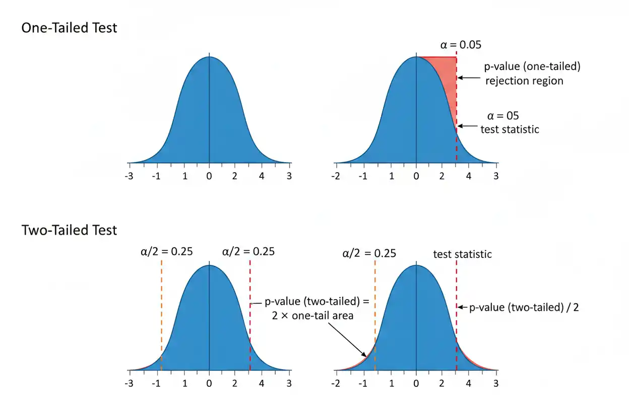
P-values are inferential statistics used to quantify how incompatible observed data are with a specified null hypothesis and statistical model. More precisely, a p-value is the probability, calculated under the null hypothesis and the assumptions of the test, of obtaining a test statistic at least as extreme as the one observed in the direction or directions specified by the test. Small p-values indicate that the observed result would be relatively unusual if the null model were correct, while large p-values indicate that the observed statistic is not especially unusual under that model. A p-value does not give the probability that the null hypothesis is true, does not measure effect size, and does not by itself determine whether a finding is practically important. Its calculation depends on the test statistic, reference distribution, and whether the alternative hypothesis is one-sided or two-sided. When a significance level α is chosen in advance, a result with p ≤ α is conventionally called statistically significant and provides grounds to reject H₀ under the stated procedure. A result with p > α means the procedure fails to reject H₀; it does not prove H₀ is true.
P-values belong to statistical inference within core statistics and the broader Statistics & Probability framework. Their calculation often relies on reference distributions such as the normal distribution, while their interpretation must remain separate from descriptive concepts such as outliers and from probability representations such as odds formats.
What Is a P-Value?
Suppose a hypothesis test begins with a null hypothesis:
H₀
A test statistic:
T
is calculated from the observed data.
The p-value asks:
Assuming H₀ and the test model are correct, how probable is a test statistic at least as extreme as the observed one?
For an upper-tailed test, the general form is:
p = P(T ≥ t_obs | H₀)
For a lower-tailed test:
p = P(T ≤ t_obs | H₀)
For a two-sided test, extremeness is measured in both directions according to the test’s definition.
For a symmetric reference distribution, a common form is:
p = 2P(T ≥ |t_obs| | H₀)
when the standardized statistic is centered symmetrically around zero.
The exact two-sided definition can vary for asymmetric or discrete tests, so the test procedure itself determines the appropriate calculation.
What Does a Small P-Value Mean?
Suppose:
p = 0.01
This means that, under the null hypothesis and statistical assumptions used in the test, the probability of obtaining a test statistic at least as extreme as the observed statistic is:
1%
It does not mean:
There is a 1% probability H₀ is true.
It also does not mean:
There is a 99% probability H₁ is true.
Those statements reverse the conditional probability being calculated.
The p-value conditions on H₀:
P(data this extreme | H₀)
It does not calculate:
P(H₀ | data)
That distinction is fundamental.
P-Value Formula
There is no single universal algebraic formula for all p-values.
The formula depends on the reference distribution of the test statistic.
For an upper-tailed test:
p = P(T ≥ t_obs | H₀)
If F is the cumulative distribution function of T under H₀:
p = 1 − F(t_obs)
For a lower-tailed test:
p = F(t_obs)
For a symmetric two-sided test:
p = 2[1 − F(|t_obs|)]
when the statistic has a continuous distribution symmetric around zero.
Examples include z-tests and many t-tests.
P-Value Example With a z-Test
Suppose a population mean is tested using:
H₀: μ = 50
against:
H₁: μ ≠ 50
Assume:
x̄ = 52
σ = 4
n = 16
and the standard assumptions for the z-test apply.
The standard error is:
SE = σ/√n
SE = 4/√16
SE = 4/4
SE = 1
The test statistic is:
z = (x̄ − μ₀)/SE
Therefore:
z = (52 − 50)/1
z = 2
Because the alternative is two-sided, we want the probability of a standard normal statistic at least as far from zero as ±2.
Thus:
p = 2P(Z ≥ 2)
From the standard normal distribution:
P(Z ≥ 2) ≈ 0.02275
Therefore:
p ≈ 2(0.02275)
p ≈ 0.04550
So:
p ≈ 0.0455
Interpreting the Example
If the significance level was chosen as:
α = 0.05
then:
p ≈ 0.0455 < 0.05
Therefore, the result is statistically significant at the 5% level.
The formal decision is:
Reject H₀
under the test procedure.
A careful interpretation is:
If μ = 50 and the test assumptions hold, a standardized result at least as extreme as the observed one would occur with probability about 4.55%.
It would be incorrect to say:
“There is a 4.55% chance that μ = 50.”
The test does not calculate that probability.
Significance Level α
The significance level:
α
is a threshold selected before examining the test result under a well-designed analysis.
Common choices include:
α = 0.05
α = 0.01
α = 0.10
The decision rule is conventionally:
If p ≤ α → reject H₀
If p > α → fail to reject H₀
For example:
p = 0.03
is statistically significant at:
α = 0.05
but not at:
α = 0.01
Statistical significance therefore depends partly on the preselected decision threshold.
P-Value vs Alpha
P-value and α play different roles.
The p-value is calculated from the observed data.
Alpha is the preselected Type I error threshold for the testing procedure.
Suppose:
p = 0.04
At:
α = 0.05
the result is significant.
At:
α = 0.01
it is not.
The observed data and p-value have not changed.
Only the decision rule has changed.
This is why reporting the actual p-value is usually more informative than reporting only:
significant
or:
not significant.
Why Alpha Should Be Chosen Before Seeing the Result
Suppose an analyst obtains:
p = 0.073
and then changes the threshold from:
α = 0.05
to:
α = 0.10
because the first threshold did not produce significance.
That practice makes the claimed error-control procedure difficult to interpret.
A significance threshold should normally be specified based on the study design, consequences of errors, and analytical plan rather than selected retrospectively to match the observed p-value.
The same principle applies to choosing between one-sided and two-sided alternatives.
One-Sided P-Values
Suppose the hypotheses are:
H₀: μ = 50
H₁: μ > 50
Using the previous example:
z = 2
Now only the upper tail is relevant.
Therefore:
p = P(Z ≥ 2)
p ≈ 0.02275
Thus:
One-sided p ≈ 0.0228
This is half the two-sided value because the standard normal distribution is symmetric and the observed z-statistic is in the direction specified by H₁.
Two-Sided P-Values
For:
H₀: μ = 50
H₁: μ ≠ 50
extreme deviations in either direction matter.
With:
z = 2
the two-sided p-value is:
p = P(Z ≤ −2) + P(Z ≥ 2)
By symmetry:
p = 2P(Z ≥ 2)
p ≈ 0.0455
A two-sided test therefore accounts for evidence both above and below the null value.
One-Sided Tests Must Be Directional in Advance
A one-sided test should not generally be chosen after observing which direction the data moved.
Suppose the scientific question genuinely concerns only:
μ > μ₀
Then a one-sided alternative can be appropriate.
But if either an increase or decrease would matter, the alternative should be:
μ ≠ μ₀
Choosing the favorable direction after seeing the sample effectively changes the testing procedure and can inflate false-positive risk.
The direction should follow the research question rather than the result.
P-Values From a t-Test
When a population standard deviation is unknown and estimated from sample data, a t-statistic is often used.
A one-sample t-statistic is:
t = (x̄ − μ₀)/(s/√n)
Under the standard one-sample t-test assumptions and H₀:
t
follows a Student’s t reference distribution with:
df = n − 1
Suppose:
t = 2.50
and:
df = 9
For a two-sided test:
p = 2P(T₉ ≥ 2.50)
which is approximately:
p ≈ 0.0339
At:
α = 0.05
this would be statistically significant.
Degrees of Freedom Matter
A t-statistic of:
2.0
does not always produce the same p-value.
The result depends on degrees of freedom.
A t distribution with few degrees of freedom has heavier tails than the standard normal distribution.
Therefore, the same absolute statistic usually produces a larger p-value when degrees of freedom are small.
As:
df → ∞
the t distribution approaches:
N(0,1)
and t-based probabilities approach corresponding normal probabilities.
P-Values From a Chi-Square Statistic
Some tests use a chi-square reference distribution.
Suppose:
χ² = 6.0
with:
df = 2
The relevant p-value is the upper-tail probability:
p = P(χ²₂ ≥ 6)
which is approximately:
p ≈ 0.0498
The right tail is used because larger chi-square statistics generally represent greater departure from the null model in standard chi-square tests.
Unlike z and t distributions, chi-square distributions are not symmetric around zero.
Therefore, simply doubling one tail would not be the appropriate method.
P-Values From Discrete Probability Models
P-values can also arise from discrete distributions.
Suppose under H₀:
X ~ Poisson(4)
and the observed count is:
X = 8
For an upper-tailed test, the p-value is:
p = P(X ≥ 8 | λ = 4)
Using the Poisson distribution:
p = 1 − P(X ≤ 7)
This gives approximately:
p ≈ 0.0511
At:
α = 0.05
the result would narrowly fail to reach the conventional 5% significance threshold.
The difference between:
0.049
and:
0.051
is mathematically small, which is one reason results near arbitrary thresholds should not be interpreted as fundamentally different scientific realities.
Discrete P-Values Behave Differently
With continuous test statistics, exact p-values under H₀ can often have a uniform distribution between 0 and 1 when the null hypothesis is simple and the test is correctly calibrated.
Discrete tests behave differently because only certain test-statistic values are possible.
Consequently, only certain p-values may be attainable.
Exact discrete tests can therefore be conservative relative to a nominal significance level.
This is another reason p-values should be interpreted in the context of the actual testing procedure rather than as generic numerical scores.
P-Value and the Null Hypothesis
A hypothesis test typically begins with:
H₀ = null hypothesis
and:
H₁ = alternative hypothesis
The p-value is calculated assuming the null model.
A small result indicates tension between the observed statistic and H₀.
However, the p-value does not specify why the tension exists.
A small p-value can result from:
- a genuine departure from H₀,
- model assumption violations,
- dependence,
- selection bias,
- measurement problems,
- multiple testing,
- data-dependent analysis choices.
Statistical significance does not automatically validate the entire analytical design.
Failing to Reject Is Not Accepting H₀
Suppose:
p = 0.42
with:
α = 0.05
The correct decision is:
Fail to reject H₀
This does not establish:
H₀ is true.
The study may have:
- little statistical power,
- a noisy measurement,
- a small sample,
- a modest effect,
- an inappropriate test.
A large p-value means the observed statistic is not sufficiently incompatible with H₀ under the procedure to cross the rejection threshold.
It is not affirmative proof of no effect.
P-Values Do Not Measure Effect Size
Suppose Study A estimates an effect of:
0.2 units
with:
p = 0.001
Study B estimates:
10 units
with:
p = 0.08
It is incorrect to conclude automatically that Study A found the larger or more important effect.
P-values depend on both:
- estimated effect magnitude,
- uncertainty.
A very large sample can make a tiny effect highly statistically significant.
A small study can estimate a large effect imprecisely and produce a larger p-value.
Effect size and p-value must therefore be considered separately.
Effect Size Example
Suppose an estimated difference is:
0.10
with standard error:
0.01
Then:
z = 0.10/0.01
z = 10
The p-value is extremely small.
Now suppose another study estimates:
5.0
with standard error:
4.0
Then:
z = 5/4
= 1.25
The p-value is much larger.
The second estimated effect is numerically fifty times larger, yet its uncertainty is also much larger.
P-values measure standardized evidence against the null model, not raw effect magnitude.
P-Values and Sample Size
Increasing sample size commonly decreases standard errors.
For a sample mean under suitable conditions:
SE = σ/√n
Therefore, even a fixed small departure from H₀ can produce a larger standardized test statistic as n increases.
This can lead to:
very small p-values for practically trivial effects
in enormous samples.
Conversely, small samples may have insufficient precision to detect effects that matter substantively.
Sample size must therefore be considered alongside effect estimates and confidence intervals.
P-Values and Statistical Power
Statistical power is:
P(reject H₀ | a specified alternative is true)
It differs from the p-value.
A p-value is computed after observing data under H₀.
Power is a design property evaluated under an alternative scenario.
Higher power generally makes a study more capable of detecting specified departures from the null.
Power can increase with:
- larger sample size,
- larger effect size,
- lower variability,
- more efficient design,
- a larger α, though that also increases Type I error tolerance.
A non-significant result from a low-power study may provide relatively weak information about whether an important effect exists.
Type I Error
A Type I error occurs when:
H₀ is true
but the test rejects it.
The significance level α controls the long-run Type I error probability under the conditions of the test.
For:
α = 0.05
the testing procedure is designed so that the probability of rejection under the relevant null model is at most or approximately:
5%
depending on the test.
This does not mean that 5% of all significant findings are false.
That latter quantity depends on many additional factors, including how often null hypotheses are actually true.
Type II Error
A Type II error occurs when:
H₀ is false
but the testing procedure fails to reject it.
Its probability is commonly written:
β
Power is:
1 − β
Unlike Type I error, Type II error depends on the particular alternative effect being considered.
A hypothesis is not simply:
true or false with one universal β.
Power calculations require specifying a meaningful departure from H₀.
P-Values and Confidence Intervals
For many standard two-sided tests, p-values and confidence intervals are closely related.
In the z-test example:
x̄ = 52
SE = 1
A 95% confidence interval is:
x̄ ± 1.96SE
Therefore:
52 ± 1.96
giving:
(50.04, 53.96)
The null value:
μ₀ = 50
lies just outside this interval.
Correspondingly, the two-sided test produced:
p ≈ 0.0455
which is slightly below:
0.05
This equivalence occurs when the confidence interval and test use compatible assumptions and methods.
Confidence Intervals Give More Information
A p-value can tell us how incompatible the observed statistic is with a particular null value.
A confidence interval additionally shows a range of parameter values compatible with the data under the interval procedure.
For example:
Estimated difference = 8
95% CI = (1, 15)
communicates both:
- direction,
- uncertainty,
- plausible effect magnitude.
Reporting only:
p = 0.03
would omit much of that information.
This is why p-values are generally more informative when presented alongside estimates and confidence intervals.
A 95% Confidence Interval Is Not a 95% Posterior Probability
In ordinary frequentist inference, once the data are observed and the interval is calculated, the population parameter is treated as fixed.
The 95% refers to the long-run coverage procedure:
Across repeated comparable samples, approximately 95% of intervals constructed by the method contain the true parameter under the model assumptions.
It is not ordinarily interpreted as:
There is a 95% probability the fixed parameter lies inside this particular observed interval.
This distinction parallels the correct interpretation of p-values.
P-Values and Percentiles
P-values are mathematically related to cumulative probabilities and therefore to percentiles, but the concepts are not identical.
Suppose a test statistic has cumulative distribution function:
F(t)
If an observed upper-tail statistic is at the 97th percentile under H₀:
F(t_obs) = 0.97
then its upper-tail p-value is:
p = 1 − 0.97
p = 0.03
Thus, percentiles describe cumulative position, while the p-value measures relevant tail probability under the null reference distribution.
P-Values and Outliers
An observation flagged as an outlier is not automatically associated with a hypothesis-test p-value.
For example, the 1.5×IQR rule uses:
Q₁ − 1.5(IQR)
and:
Q₃ + 1.5(IQR)
as exploratory fences.
It does not produce a formal p-value.
Formal tests for unusual observations require a specified statistical model and test statistic.
Even when such a p-value is calculated, a statistically unusual observation is not automatically an erroneous observation.
P-Values and Odds
A p-value should not be converted through odds formats and interpreted as odds that the null hypothesis is true.
Suppose:
p-value = 0.05
Mathematically converting 0.05 into:
5% probability
and then into:
19:1 odds against
would misrepresent what the p-value means.
The value 0.05 is a conditional tail probability under H₀.
It is not:
P(H₀ | data) = 0.05
Probability-to-odds conversion is appropriate only when the input quantity actually represents the probability of the event being discussed.
P-Values Are Not the Probability the Result Happened by Chance
Another common phrase is:
“The probability that the result was due to chance is p.”
That is generally inaccurate.
The p-value asks about data extremeness assuming a specified null model.
It does not divide possible explanations into:
chance
versus:
not chance
and calculate probabilities for those explanations.
Random variation is built into the reference model, but the p-value does not provide a posterior probability that chance “caused” the observed result.
P-Values Do Not Measure Reproducibility
A small p-value does not guarantee that another study will obtain:
- the same estimate,
- the same direction,
- another significant result.
Replication depends on:
- true effect size,
- study power,
- measurement reliability,
- sampling variation,
- research design,
- publication and selection processes.
Two statistically valid studies can produce different p-values simply because they sampled different observations.
P-values are random quantities that vary from sample to sample.
The Same Effect Can Produce Different P-Values
Suppose two studies estimate the same effect:
2 units
Study A has:
SE = 0.5
so:
statistic = 2/0.5 = 4
Study B has:
SE = 2
so:
statistic = 2/2 = 1
Their p-values will differ substantially even though the point estimates are identical.
The reason is uncertainty.
A p-value cannot therefore be interpreted without considering standard errors and study precision.
P = 0.05 Is Not a Scientific Boundary
The difference between:
p = 0.049
and:
p = 0.051
is tiny.
Yet a rigid threshold at:
α = 0.05
can label the first:
statistically significant
and the second:
not statistically significant.
That categorical difference should not be mistaken for a large difference in evidence.
Exact p-values, confidence intervals, effect estimates, and study design should be considered together.
P = 0.000 Does Not Mean Zero Probability
Statistical software may display:
p = 0.000
because of limited decimal precision.
The actual p-value is usually:
very small but positive.
For example, software displaying three decimals may show 0.000 for:
p = 0.00021
The appropriate report is something such as:
p < 0.001
rather than:
p = 0
unless the exact mathematical probability is genuinely zero, which is unusual in ordinary continuous hypothesis testing.
Large P-Values Are Not Evidence of Exact Equality
Suppose a test of:
H₀: μ₁ − μ₂ = 0
produces:
p = 0.80
This does not prove:
μ₁ = μ₂
exactly.
The data may simply be compatible with a broad range of differences.
If the real scientific goal is to demonstrate that two effects are sufficiently similar, methods such as equivalence testing may be more appropriate than a conventional null-hypothesis test of exact equality.
Failure to detect a difference is not automatically evidence of equivalence.
Multiple Testing
Suppose many hypotheses are tested independently at:
α = 0.05
Even when all null hypotheses are true, the probability of at least one false rejection grows as the number of tests increases.
For m independent tests:
P(at least one Type I error) = 1 − (1 − α)^m
For:
m = 20
and:
α = 0.05
we obtain:
1 − 0.95²⁰
≈ 0.6415
Therefore, the chance of at least one false positive is approximately:
64.15%
under these simplifying independence conditions.
This illustrates why multiple-testing adjustments can be important.
Bonferroni Adjustment
One simple method for controlling family-wise Type I error is the Bonferroni adjustment.
If the desired family-wise level is:
α
and m hypotheses are tested, each test can use:
α_adjusted = α/m
For:
α = 0.05
and:
m = 10
we obtain:
α_adjusted = 0.005
This procedure can be conservative, particularly when tests are correlated or numerous.
Other multiple-testing procedures may provide more power while controlling different error criteria.
P-Hacking
P-hacking refers broadly to analytical behavior that increases the chance of obtaining a favorable small p-value through repeated or data-dependent choices.
Examples can include repeatedly changing:
- exclusion criteria,
- outcome definitions,
- covariates,
- stopping points,
- subgroups,
- one- versus two-sided tests,
until statistical significance appears.
Such practices invalidate the simple nominal interpretation of the final p-value because the reported test no longer reflects the full selection process.
Pre-specification and transparent reporting help protect inferential validity.
Optional Stopping
Suppose data are repeatedly examined and sampling stops as soon as:
p < 0.05
A conventional fixed-sample p-value may no longer provide the intended Type I error control unless the sequential design is accounted for.
Repeated opportunities to stop when results look favorable alter the probability of eventually crossing the threshold.
Sequential testing methods can properly incorporate planned interim analyses.
The stopping rule is therefore part of the statistical design.
Model Assumptions Matter
A mathematically precise p-value can still be misleading if its test model is inappropriate.
Possible problems include:
- dependent observations,
- wrong distributional assumptions,
- nonconstant variance,
- incorrect functional form,
- biased sampling,
- measurement error.
The p-value is conditional on the statistical procedure being suitable.
Checking model assumptions is therefore not optional merely because the final number has many decimal places.
Independence
Many standard hypothesis tests rely on independent observations or on a correctly specified dependence model.
If observations are clustered or repeated but treated as independent, conventional standard errors can be too small.
This can produce test statistics that are too large and p-values that are misleadingly small.
Examples include:
- repeated measurements from the same person,
- students nested within classrooms,
- time-series observations,
- multiple measurements from one device.
The sampling structure determines the appropriate analysis.
Normality Assumptions
Some classical tests derive exact small-sample reference distributions under normal error assumptions.
This does not mean every raw variable must always be normally distributed.
The relevant assumption depends on the test.
For large samples, some procedures can be approximately valid under broader conditions because of asymptotic theory.
However, severe skewness, heavy tails, extreme observations, or small samples can still matter.
The test assumptions should be identified specifically rather than summarized as:
“The data must be normal.”
Statistical Significance vs Practical Significance
Suppose a very large study estimates that a treatment changes a measurement by:
0.02 units
with:
p < 0.001
The result is statistically significant.
But if a change smaller than:
1 unit
has no practical consequence, the effect may be substantively negligible.
Conversely, an estimated improvement of:
5 units
with:
p = 0.08
may be potentially important but imprecisely estimated.
Statistical and practical significance answer different questions.
Statistical Significance vs Causation
A small p-value does not prove causation.
Suppose two observational variables are strongly associated and produce:
p < 0.001
Possible explanations include:
- causal effect,
- reverse causation,
- confounding,
- selection,
- common trends,
- measurement artifacts.
The p-value evaluates a test statistic under a null model.
Causal conclusions require an appropriate research design and identification assumptions beyond statistical significance.
Statistical Significance vs Importance
A p-value does not tell us whether the research question itself is important.
A statistically significant relationship can be:
- tiny,
- obvious,
- poorly measured,
- unimportant operationally.
Likewise, a non-significant result can concern an extremely important parameter for which the study simply lacked precision.
Interpretation should therefore combine statistical evidence with substantive context.
P-Value Distribution Under H₀
For a correctly calibrated continuous test under a simple null hypothesis, the p-value has a uniform distribution on:
[0,1]
under H₀.
Therefore:
P(p ≤ 0.05 | H₀) = 0.05
This is the basis of the conventional Type I error interpretation.
It also means that when H₀ is true, very large p-values are not inherently more “correct” than moderate ones.
Values throughout the interval are expected.
Discrete and composite-null settings can modify this exact uniformity.
P-Values Under an Alternative
When a meaningful alternative hypothesis is true and the test has power, p-values tend to be concentrated closer to zero.
The degree of concentration depends on:
- effect size,
- sample size,
- variability,
- test efficiency.
A strong effect in a large precise study often produces a very small p-value.
A weak effect or noisy small sample may produce a large one even when H₀ is false.
Thus, the p-value distribution depends on both the underlying effect and study design.
Reporting P-Values
A useful report typically includes more than the p-value.
For example:
Mean difference = 2.0 units, 95% CI = 0.04 to 3.96, z = 2.00, p = 0.0455.
This communicates:
- effect estimate,
- uncertainty,
- test statistic,
- p-value.
Reporting only:
p < 0.05
loses information about both evidence and effect magnitude.
Exact values are often preferable unless they are extremely small.
Common P-Value Mistakes
A common mistake is saying:
“p = 0.03 means H₀ has a 3% probability of being true.”
That is incorrect.
Another is saying:
“p = 0.03 means there is a 3% probability the result happened by chance.”
That is also generally incorrect.
Another error is treating:
p > 0.05
as proof of no effect.
Analysts also frequently equate statistical significance with practical importance or causation.
Another mistake is switching to a one-sided test after seeing the direction of the data.
Running many analyses and reporting only the smallest p-value without adjustment is another serious problem.
It is also incorrect to interpret:
p = 0.000
from software as a mathematically zero probability.
Finally, p-values should not be interpreted without considering effect size, uncertainty, assumptions, sample size, and study design.
How to Calculate a P-Value Step by Step
A reliable hypothesis-test procedure follows these stages.
Step 1: State the Null Hypothesis
For example:
H₀: μ = 50
Step 2: State the Alternative
Two-sided:
H₁: μ ≠ 50
Upper-tailed:
H₁: μ > 50
Lower-tailed:
H₁: μ < 50
Step 3: Choose the Test Statistic
Examples include:
z
t
χ²
F
or a discrete probability statistic.
Step 4: Calculate the Observed Statistic
Use the formula required by the test.
Step 5: Determine the Reference Distribution Under H₀
For example:
Standard normal
Student’s t with specified df
Chi-square with specified df
Poisson with specified λ
Step 6: Calculate the Appropriate Tail Probability
The alternative hypothesis determines whether the test is:
- lower-tailed,
- upper-tailed,
- two-sided.
Step 7: Compare p With α
If:
p ≤ α
reject H₀ under the test procedure.
Otherwise:
fail to reject H₀.
Step 8: Interpret the Effect
Report:
- estimate,
- uncertainty,
- substantive importance,
- assumptions,
rather than stopping at the significance decision.
Full Worked Example
Suppose a process is claimed to have population mean:
μ = 100
A sample produces:
x̄ = 104
Assume:
σ = 12
n = 36
and the assumptions for a two-sided z-test hold.
Test:
H₀: μ = 100
H₁: μ ≠ 100
Calculate the Standard Error
SE = σ/√n
SE = 12/6
SE = 2
Calculate z
z = (104 − 100)/2
z = 2
Calculate the Two-Sided P-Value
p = 2P(Z ≥ 2)
p ≈ 0.0455
Compare With Alpha
For:
α = 0.05
we have:
0.0455 < 0.05
Therefore:
Reject H₀
at the 5% significance level.
Interpret
A suitable statement is:
Under H₀: μ = 100 and the assumptions of the z-test, a sample result producing a statistic at least as extreme as z = ±2 would occur with probability approximately 4.55%.
That is the meaning of the p-value.
Frequently Asked Questions About P-Values
What are p-values?
P-values are probabilities calculated under a null hypothesis that measure how extreme the observed test statistic is relative to its null reference distribution.
What is the basic p-value formula?
For an upper-tailed test:
p = P(T ≥ t_obs | H₀)
For a lower-tailed test:
p = P(T ≤ t_obs | H₀)
The exact two-sided formula depends on the test.
What does p = 0.05 mean?
It means that under H₀ and the test assumptions, outcomes at least as extreme as the observed statistic occur with probability 5% according to the test’s definition of extremeness.
Does p = 0.05 mean H₀ has a 5% probability of being true?
No.
Does p = 0.01 mean there is a 99% probability H₁ is true?
No.
What does a small p-value indicate?
It indicates that the observed test statistic is relatively incompatible with the null model.
What does a large p-value indicate?
It means the observed statistic is not especially unusual under H₀. It does not prove H₀.
What is alpha?
Alpha is the preselected significance threshold used for a hypothesis-test decision.
What happens if p ≤ α?
The null hypothesis is rejected under the specified testing procedure.
What happens if p > α?
The test fails to reject H₀.
Is failing to reject the same as accepting H₀?
No. Failure to reject is not proof that H₀ is true.
What is the difference between one-sided and two-sided p-values?
A one-sided p-value examines extremeness in one pre-specified direction. A two-sided p-value accounts for departures in both directions.
Can I choose a one-sided test after seeing the result?
That generally invalidates the intended error rate. The direction should be determined by the research question before examining the outcome.
Does a smaller p-value mean a larger effect?
No. P-values depend on effect size, uncertainty, and sample size.
Does a statistically significant result have practical importance?
Not necessarily. Statistical significance and practical significance are different.
Does a small p-value prove causation?
No. Causal conclusions require appropriate study design and assumptions.
Can an enormous sample make a tiny effect significant?
Yes. Large samples can produce small standard errors, making very small departures from H₀ statistically detectable.
Can a meaningful effect have p > 0.05?
Yes. Small or noisy studies can estimate important effects imprecisely.
How are p-values related to confidence intervals?
For many compatible two-sided procedures, a null value rejected at α = 0.05 lies outside the corresponding 95% confidence interval.
Is a p-value the same as a confidence level?
No. They are related through inferential procedures but represent different quantities.
Is a p-value a percentile?
Not exactly. A p-value is a tail probability under a null reference distribution, while a percentile describes cumulative position. The two can be mathematically related through the distribution’s CDF.
Can the normal distribution be used to calculate p-values?
Yes. z-tests and many asymptotic procedures use standard normal reference probabilities.
Can discrete distributions produce p-values?
Yes. Tests can use distributions such as the Poisson distribution, binomial distribution, or other discrete reference models.
Why can discrete p-values behave differently?
A discrete statistic can take only certain values, so the attainable p-values are also discrete rather than continuously spread over 0 to 1.
Is an outlier automatically statistically significant?
No. Exploratory outlier rules and formal hypothesis-test p-values are different concepts.
Can a p-value be converted to odds that H₀ is true?
No, not under the ordinary frequentist interpretation. A p-value is not P(H₀ | data).
What does p = 0.000 mean in software?
Usually it means the value is smaller than the display precision, not literally zero.
What is multiple testing?
Multiple testing occurs when many hypotheses are tested. Without adjustment, the probability of at least one false-positive rejection can increase substantially.
What is p-hacking?
It refers to data-dependent analytical choices made in ways that increase the chance of obtaining a small reported p-value.
Should p-values be reported alone?
Usually not. Effect estimates, confidence intervals, sample size, assumptions, and substantive interpretation provide essential additional information.
Is p = 0.049 meaningfully different from p = 0.051?
The numerical evidence is very similar. A significance threshold may classify them differently, but they should not be treated as fundamentally different scientific results.
What is the safest interpretation of a p-value?
Interpret it as a tail probability under the specified null model and test assumptions, then evaluate it together with effect magnitude, uncertainty, study design, statistical power, and practical relevance.




