Normal Distribution: Definition, Formula & Example

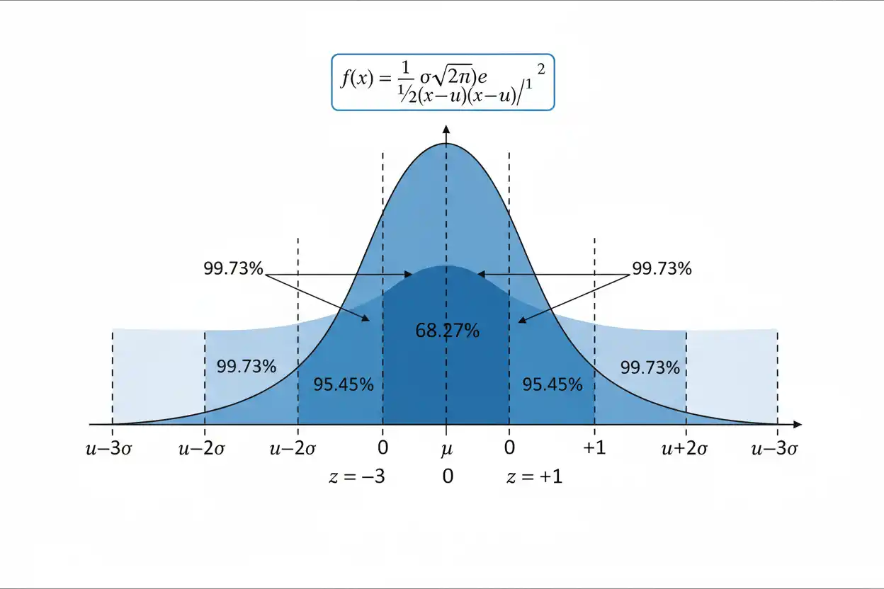
The normal distribution is a continuous probability distribution defined by a symmetric, bell-shaped density centered on its mean. It is one of the most important probability models in statistics because many measurements are approximately normal under suitable conditions, many estimation procedures use normal or approximately normal sampling distributions, and standardized normal probabilities appear throughout confidence intervals and hypothesis testing. A normal distribution is completely determined by two parameters: the population mean μ, which controls its center, and the population standard deviation σ, which controls its spread. Its variance is σ², its total probability equals 1, and exactly half of its probability lies on each side of μ because the distribution is symmetric. Individual points have probability zero because the normal distribution is continuous; probabilities correspond to areas under the density curve over intervals. Any normally distributed variable can also be standardized into a z-score, allowing probabilities for different normal distributions to be evaluated using the standard normal distribution. Although the familiar 68–95–99.7 rule provides useful approximations, accurate probability calculations use the normal cumulative distribution function rather than treating the empirical rule as exact for arbitrary intervals.

The normal distribution is a central probability model within core statistics and the broader Statistics & Probability framework. Its two parameters connect naturally with mean and variance, while its symmetry explains the familiar relationship among mean, median, mode in an ideal normal population.

What Is a Normal Distribution?

A normal distribution is a continuous probability distribution with a density function that is symmetric around its population mean.

If:

X ~ N(μ, σ²)

then X follows a normal distribution with:

Mean = μ

Variance = σ²

Standard deviation = σ

where:

σ > 0

The notation:

N(μ, σ²)

uses the variance as the second parameter.

For example:

X ~ N(100, 15²)

means:

μ = 100

and:

σ = 15

so:

Var(X) = 225

The mean determines where the normal curve is centered, while the standard deviation determines how widely probability is spread around that center.

Normal Distribution Formula

The probability density function is:

f(x) = [1/(σ√(2π))]e^[−(x − μ)²/(2σ²)]

where:

• x = possible value of the continuous variable
• μ = population mean
• σ = population standard deviation
• σ² = population variance
• π ≈ 3.14159
• e ≈ 2.71828

The density is defined for every real number:

−∞ < x < ∞

and:

σ > 0

The formula determines the familiar bell-shaped curve.

What the Normal Distribution Formula Means

The expression:

(x − μ)²

measures squared distance from the center.

Because it is squared, observations equally far above and below μ receive the same density.

The denominator:

2σ²

controls how quickly the exponential term declines as x moves away from μ.

A larger σ causes the density to decline more slowly, producing a wider curve.

A smaller σ concentrates probability more tightly around μ.

The factor:

1/(σ√(2π))

scales the curve so that its total area equals exactly:

1

Therefore:

∫ from −∞ to ∞ f(x) dx = 1

Why the Normal Distribution Is Bell-Shaped

At:

x = μ

the squared deviation is zero:

(x − μ)² = 0

Therefore, the exponential factor becomes:

e⁰ = 1

and the density reaches its maximum:

f(μ) = 1/(σ√(2π))

As x moves away from μ in either direction, the squared deviation increases.

The exponent becomes increasingly negative, causing the density to fall smoothly toward zero.

Because the squared distance is the same for μ + d and μ − d:

f(μ + d) = f(μ − d)

The result is a symmetric bell-shaped normal distribution.

Mean of a Normal Distribution

If:

X ~ N(μ, σ²)

then:

E(X) = μ

The parameter μ therefore identifies the population arithmetic mean.

Changing μ shifts the entire normal distribution horizontally.

For example:

N(0, 1)

is centered at zero, while:

N(50, 1)

has exactly the same shape but is centered at 50.

Changing the mean does not by itself alter the distribution’s spread.

Variance of a Normal Distribution

For:

X ~ N(μ, σ²)

the variance is:

Var(X) = σ²

and the standard deviation is:

SD(X) = σ

The variance controls the squared spread around μ.

For example:

X ~ N(100, 25)

means:

μ = 100

σ² = 25

σ = 5

It is important not to read the second normal-distribution parameter as the standard deviation when the notation explicitly uses:

N(μ, σ²)

The convention should always be checked because some software interfaces request σ directly rather than σ².

Mean, Median, and Mode

For an ideal normal distribution:

Mean = Median = Mode = μ

The mean equals μ by definition.

Symmetry places the median at μ because:

P(X ≤ μ) = 0.5

and:

P(X ≥ μ) = 0.5

The density also reaches its unique maximum at μ, making μ the mode.

Therefore:

Mean = Median = Mode

for every nondegenerate normal distribution.

This equality is a distinctive property of the symmetric unimodal normal model and should not be generalized to skewed distributions.

Symmetry of the Normal Distribution

The normal distribution is perfectly symmetric around μ.

For any positive distance d:

P(μ − d ≤ X ≤ μ) = P(μ ≤ X ≤ μ + d)

Likewise:

P(X < μ − d) = P(X > μ + d)

For example, the probability of being more than two standard deviations below the mean equals the probability of being more than two standard deviations above the mean.

This symmetry simplifies many calculations because one tail can often be obtained from the other.

Total Area Under the Curve

Because the normal distribution is a probability distribution:

Total area = 1

Therefore:

P(−∞ < X < ∞) = 1

Since the curve is symmetric:

P(X < μ) = 0.5

and:

P(X > μ) = 0.5

For a continuous distribution, using:

<

or:

≤

at a single exact boundary does not change the probability because:

P(X = a) = 0

for every individual real value a.

Probability at a Single Point

A common misconception is to interpret the density height as the probability of observing exactly x.

For a continuous normal distribution:

P(X = x) = 0

for every exact x.

This does not mean the value is impossible.

It means that probability is assigned to intervals rather than individual points.

For example:

P(70 ≤ X ≤ 71)

can be positive.

But:

P(X = 70)

equals zero mathematically under a continuous model.

Density Is Not Probability

The value:

f(x)

is a probability density, not a probability.

Probability over an interval is the area:

P(a ≤ X ≤ b) = ∫ from a to b f(x) dx

The density can even exceed 1 when σ is sufficiently small.

That does not violate probability rules because the total area, not the density height, must equal 1.

This distinction is essential when interpreting continuous probability distributions.

Standard Normal Distribution

The standard normal distribution is the special normal distribution with:

μ = 0

and:

σ = 1

It is commonly represented by:

Z ~ N(0,1)

The standard normal density is:

φ(z) = [1/√(2π)]e^(−z²/2)

Any normally distributed observation can be converted to the standard normal scale using a z-score.

This allows one common probability distribution to represent every possible normal distribution after standardization.

What Is a z-Score?

A z-score measures how many standard deviations an observation lies above or below the mean.

The formula is:

z = (x − μ)/σ

where:

• x = observed value
• μ = population mean
• σ = population standard deviation
• z = standardized score

If:

z = 0

then:

x = μ

If:

z = 1

the observation lies one standard deviation above the mean.

If:

z = −2

the observation lies two standard deviations below the mean.

z-Score Example

Suppose:

X ~ N(70, 10²)

and an observation is:

x = 85

Calculate:

z = (85 − 70)/10

z = 15/10

z = 1.5

Therefore, 85 lies:

1.5 standard deviations above the mean.

The original measurement scale has now been converted into a standardized scale.

Standardizing Does Not Change Relative Position

Suppose two different examinations use different scoring scales.

Exam A:

μ = 60

σ = 8

A student scores:

72

Then:

z = (72 − 60)/8

z = 1.5

Exam B:

μ = 500

σ = 100

A student scores:

650

Then:

z = (650 − 500)/100

z = 1.5

The raw scores are very different, but both observations occupy the same standardized position relative to their respective distributions.

Converting a z-Score Back to x

Start with:

z = (x − μ)/σ

Multiply by σ:

zσ = x − μ

Then:

x = μ + zσ

This formula converts a standardized position back to the original measurement scale.

For example, if:

μ = 100

σ = 15

and:

z = 1.5

then:

x = 100 + 1.5(15)

x = 122.5

Normal Cumulative Distribution Function

The cumulative distribution function of a normal variable gives:

P(X ≤ x)

For a standard normal variable, the CDF is commonly written:

Φ(z) = P(Z ≤ z)

Unlike the density function, the normal CDF does not have a simple elementary closed-form expression.

Probability tables and statistical software evaluate it numerically.

For example:

Φ(0) = 0.5

Φ(1) ≈ 0.8413

Φ(1.5) ≈ 0.9332

Φ(2) ≈ 0.9772

These values represent cumulative area to the left of each z-score.

Normal Distribution Probability Example

Suppose:

X ~ N(70, 10²)

Find:

P(X ≤ 85)

First calculate the z-score:

z = (85 − 70)/10

z = 1.5

Therefore:

P(X ≤ 85) = P(Z ≤ 1.5)

Using the standard normal CDF:

Φ(1.5) ≈ 0.9332

Thus:

P(X ≤ 85) ≈ 0.9332

or approximately:

93.32%

About 93.32% of the normal distribution lies at or below 85.

Upper-Tail Probability

Using the same model:

X ~ N(70, 10²)

find:

P(X > 85)

Because total probability equals 1:

P(X > 85) = 1 − P(X ≤ 85)

Therefore:

P(X > 85) = 1 − 0.9332

P(X > 85) ≈ 0.0668

So approximately:

6.68%

of the distribution lies above 85.

Probability Between Two Values

For:

X ~ N(70, 10²)

find:

P(60 ≤ X ≤ 80)

Standardize the lower bound:

z₁ = (60 − 70)/10

z₁ = −1

Standardize the upper bound:

z₂ = (80 − 70)/10

z₂ = 1

Therefore:

P(60 ≤ X ≤ 80) = P(−1 ≤ Z ≤ 1)

Using standard normal probabilities:

Φ(1) ≈ 0.8413

Φ(−1) ≈ 0.1587

Subtract:

0.8413 − 0.1587

≈ 0.6827

Thus:

P(60 ≤ X ≤ 80) ≈ 68.27%

Probability Outside an Interval

Suppose:

X ~ N(70, 10²)

Find:

P(X < 50 or X > 90)

The two boundaries correspond to:

z = −2

and:

z = 2

Therefore:

P(|Z| > 2)

Using symmetry:

P(|Z| > 2) = 2P(Z > 2)

Since:

P(Z > 2) ≈ 0.0228

we obtain:

P(|Z| > 2) ≈ 0.0455

Therefore, approximately:

4.55%

of a normal distribution lies more than two standard deviations from its mean.

The 68–95–99.7 Rule

The empirical rule summarizes three important areas of a normal distribution.

Approximately:

68.27%

of observations lie within:

μ ± 1σ

Approximately:

95.45%

lie within:

μ ± 2σ

Approximately:

99.73%

lie within:

μ ± 3σ

These are often rounded to:

68%

95%

99.7%

The rule is useful for mental estimates, but exact normal probabilities differ slightly from these rounded values.

Within One Standard Deviation

For:

X ~ N(μ, σ²)

the interval:

μ − σ ≤ X ≤ μ + σ

contains approximately:

68.27%

of the probability.

The two tails therefore contain approximately:

31.73%

combined.

Because of symmetry, each tail contains about:

15.87%

This is why a z-score of:

1

has cumulative probability approximately:

0.8413

Within Two Standard Deviations

The interval:

μ − 2σ ≤ X ≤ μ + 2σ

contains approximately:

95.45%

of a normal distribution.

Therefore, probability outside that interval is approximately:

4.55%

or about:

2.275%

in each tail.

This result is close to—but not exactly—the familiar 95% interval based on:

z = ±1.96

The 1.96 cutoff encloses approximately exactly 95% rather than the approximately 95.45% enclosed by ±2.

Within Three Standard Deviations

The interval:

μ − 3σ ≤ X ≤ μ + 3σ

contains approximately:

99.73%

of a normal distribution.

Only about:

0.27%

lies outside.

Each tail contains approximately:

0.135%

This explains why observations more than three standard deviations from the mean can appear unusual under a normal model.

However, an unusual standardized value should not automatically be classified as erroneous or deleted.

Detailed treatment of unusual observations belongs with outliers, where model assumptions and context matter as much as distance from the mean.

Normal Distribution Percentiles

A percentile identifies the value below which a specified proportion of the distribution lies.

Suppose:

X ~ N(μ, σ²)

and we want the p-th cumulative quantile.

First find the standard normal z-value satisfying:

Φ(zp) = p

Then transform back:

xp = μ + zpσ

This procedure converts a standard-normal percentile to the original measurement scale.

95th Percentile Example

Suppose:

X ~ N(100, 15²)

Find the 95th percentile.

The standard normal 95th percentile is approximately:

z0.95 ≈ 1.645

Therefore:

x0.95 = 100 + 1.645(15)

x0.95 = 100 + 24.675

x0.95 ≈ 124.675

Thus, the 95th percentile is approximately:

124.7

About 95% of the modeled population lies below this value and about 5% lies above it.

25th and 75th Percentiles

For the standard normal distribution:

z0.25 ≈ −0.6745

and:

z0.75 ≈ 0.6745

Therefore, for:

X ~ N(μ, σ²)

the first quartile is approximately:

Q₁ = μ − 0.6745σ

and the third quartile is:

Q₃ = μ + 0.6745σ

The interquartile range is therefore approximately:

IQR = 1.349σ

for a normal population.

This relationship is specific to the normal distribution rather than a universal relationship between IQR and standard deviation.

Shape and the Standard Deviation

Changing σ alters the shape while preserving total area.

Suppose two normal distributions have the same mean.

Distribution A:

σ = 2

Distribution B:

σ = 10

Distribution A is narrower and taller because its probability is concentrated closer to μ.

Distribution B is wider and lower because the same total probability of 1 is spread over a larger range.

A larger standard deviation therefore means greater dispersion, not greater total probability.

Inflection Points

The normal density changes curvature at:

x = μ − σ

and:

x = μ + σ

These are the inflection points of the bell curve.

Between them, the curve has one curvature pattern.

Beyond them, the curvature reverses as the tails flatten toward the horizontal axis.

Thus, the standard deviation affects not only probability spread but also characteristic geometric features of the density.

The Tails Never Reach Zero

The normal density approaches zero as:

x → ±∞

but never actually reaches zero at any finite x.

Therefore, the theoretical support is:

(−∞, ∞)

Every finite interval in the far tail has some positive probability, however small.

This is mathematically convenient but can be unrealistic for variables that have strict physical bounds.

For example, a normal model for a quantity that cannot be negative technically assigns some probability to negative values unless μ is sufficiently far above zero relative to σ.

Model suitability must therefore consider the real measurement domain.

Standardizing the Entire Distribution

If:

X ~ N(μ, σ²)

define:

Z = (X − μ)/σ

Then:

Z ~ N(0,1)

The mean transforms as:

E(Z) = 0

and the variance becomes:

Var(Z) = 1

This transformation preserves probability ordering.

For any x:

P(X ≤ x) = P[Z ≤ (x − μ)/σ]

Standardization is therefore the bridge between a general normal distribution and standard normal probability calculations.

Linear Transformations of a Normal Variable

If:

X ~ N(μ, σ²)

and:

Y = aX + b

then:

Y ~ N(aμ + b, a²σ²)

provided:

a ≠ 0

The transformed mean is:

E(Y) = aμ + b

The transformed variance is:

Var(Y) = a²σ²

For example, if:

X ~ N(10, 4)

so:

μ = 10

σ² = 4

and:

Y = 3X + 5

then:

E(Y) = 3(10) + 5

= 35

and:

Var(Y) = 3²(4)

= 36

Therefore:

Y ~ N(35, 36)

Sums of Independent Normal Variables

If:

X ~ N(μX, σX²)

and:

Y ~ N(μY, σY²)

are independent, then:

X + Y

is also normally distributed.

Specifically:

X + Y ~ N(μX + μY, σX² + σY²)

For example:

X ~ N(10, 4)

Y ~ N(20, 9)

independently.

Then:

X + Y ~ N(30, 13)

This closure under addition is one reason the normal distribution is mathematically convenient.

Difference of Independent Normal Variables

If X and Y are independent normal variables, then:

X − Y

is also normal.

The mean is:

E(X − Y) = μX − μY

The variance is:

Var(X − Y) = σX² + σY²

because:

Var(−Y) = Var(Y)

For dependent variables, covariance terms must be included.

Independence is therefore important when simply adding the variances.

Sample Means and the Normal Distribution

Suppose:

X₁, X₂, …, Xₙ

are independent observations from:

N(μ, σ²)

Then the sample mean:

X̄

is exactly normally distributed:

X̄ ~ N(μ, σ²/n)

Its standard deviation is:

σ/√n

Thus, averaging normally distributed independent observations preserves normality while reducing spread.

This exact result should be distinguished from the central limit theorem, which can produce approximate normality for sample means even when the original observations are not normal.

Normal Distribution vs Central Limit Theorem

The central limit theorem does not say that all large data sets become normally distributed.

Instead, under suitable conditions, the distribution of a properly standardized sample mean or sum approaches a normal distribution as sample size increases.

The original population can remain skewed or discrete.

For example, individual observations may come from a non-normal population while:

X̄

has an approximately normal sampling distribution for sufficiently large n.

This distinction is fundamental.

Normality of raw data and normality of a sampling statistic are separate questions.

Not Every Bell-Shaped Distribution Is Normal

A symmetric, unimodal histogram may look approximately bell-shaped without following an exact normal distribution.

Other probability distributions can also be:

• symmetric,
• unimodal,
• centered similarly.

They can differ in:

• tail thickness,
• peak height,
• kurtosis,
• probability of extreme observations.

The normal distribution is defined by its mathematical density, not simply by visual resemblance to a bell.

Graphical and quantitative diagnostics can help determine whether a normal approximation is reasonable.

Skewness of a Normal Distribution

A theoretical normal distribution has:

Skewness = 0

because it is perfectly symmetric.

However:

sample skewness ≠ 0

does not automatically prove that the population is non-normal.

Random samples from a normal population can show some asymmetry.

The question is whether observed deviations from symmetry are larger than would reasonably be expected from sampling variation and whether those deviations matter for the intended analysis.

Kurtosis of a Normal Distribution

Under the common standardized definition, the normal distribution has:

Kurtosis = 3

and:

Excess kurtosis = 0

“Excess” kurtosis subtracts the normal benchmark of 3.

Distributions with heavier or lighter tails can have different kurtosis values.

However, sample kurtosis can be unstable, especially in small samples, because extreme observations have substantial influence.

Kurtosis should be interpreted alongside graphical evidence and other diagnostics.

Normal Probability and Odds

The normal distribution produces probabilities.

For example:

P(Z > 2) ≈ 0.0228

Probability can be converted into odds when that representation is useful.

If an event has probability:

p

its odds in favor are:

p/(1 − p)

For:

p = 0.0228

the odds in favor are approximately:

0.0228/0.9772

≈ 0.0233

Different conventions for expressing and converting odds are treated separately under odds formats. The normal distribution itself remains fundamentally a probability-density model rather than an odds model.

Normal Distribution vs Negative Binomial

The negative binomial distribution and the normal distribution model fundamentally different types of random variables.

The normal distribution is:

continuous

with support:

−∞ < x < ∞

The negative binomial is:

discrete

with integer count support.

A negative binomial model is often right-skewed, while a normal distribution is symmetric.

For suitable parameter ranges, a normal approximation to some discrete count distributions may sometimes be useful, but the approximation must be justified rather than assumed simply because counts are large.

Exact discrete probabilities are preferable when they are readily available and accuracy in the tails matters.

Normal Approximation to Discrete Data

When a discrete variable is approximated by a continuous normal distribution, a continuity correction can improve accuracy.

Suppose an integer-valued variable X is approximated by a normal variable Y.

The event:

X ≤ 10

may be approximated using:

Y ≤ 10.5

Similarly:

X ≥ 10

may correspond approximately to:

Y ≥ 9.5

The 0.5 adjustment accounts for the fact that an integer count represents a discrete probability mass occupying an interval on the continuous scale.

Whether the approximation is sufficiently accurate depends on the original distribution and its parameters.

Outliers Under a Normal Model

Because normal probabilities decline quickly in the tails, observations with large absolute z-scores can be unusual.

For example:

|z| > 3

places an observation outside the central approximately:

99.73%

of a normal distribution.

However, that does not prove the observation is an error.

In a very large data set, even rare tail events can occur naturally.

An observation can also appear extreme because the population is not actually normal.

Therefore, unusual observations should be investigated rather than automatically removed.

The Three-Sigma Rule Is Not an Automatic Deletion Rule

Suppose a sample contains an observation with:

z = 3.4

Under a genuine normal population, such a value lies in a relatively rare region.

But several explanations remain possible:

• a valid extreme observation,
• measurement error,
• data-entry error,
• mixture of subpopulations,
• heavier-than-normal tails,
• changing variance,
• model misspecification.

The normal distribution provides a probability benchmark.

It does not independently determine data quality.

Normal Distribution and Measurement Bounds

A normal distribution has infinite support in both directions.

This can be problematic when modeling a quantity that must satisfy:

X ≥ 0

If μ is large relative to σ, the probability assigned below zero may be negligibly small.

For example, a variable with:

μ = 100

σ = 5

has virtually no normal probability below zero.

But if:

μ = 5

σ = 10

a substantial portion of the normal model lies below zero.

A different probability model may be more appropriate when the physical boundary materially affects the distribution.

Normality and Sample Size

A small sample can look non-normal simply because few observations provide a noisy picture of the population.

A large sample can reveal minor deviations from normality that are statistically detectable but practically irrelevant for some procedures.

Therefore, assessing normality should not rely on a single rule.

Consider:

• sample size,
• graphical shape,
• tail behavior,
• outliers,
• the statistical method being used,
• robustness of that method to deviations.

The important question is often not:

“Is the data perfectly normal?”

but:

“Is the normal model sufficiently appropriate for the purpose?”

Histograms and Normality

A histogram can provide a useful first look.

A normal-like sample may show:

• one central peak,
• approximate symmetry,
• progressively thinner tails,
• no strong gaps or secondary clusters.

However, histogram appearance depends on bin width and sample size.

Changing bin boundaries can make the same data look quite different.

Therefore, a histogram should be combined with other diagnostics rather than treated as a definitive normality test.

Q–Q Plots

A normal Q–Q plot compares observed sample quantiles with theoretical normal quantiles.

If the sample follows a normal distribution reasonably closely, plotted points tend to lie near a straight reference line.

Systematic patterns can reveal departures:

• curved ends may indicate unusual tails,
• an S-shaped pattern may suggest tail differences,
• strong isolated deviations may indicate unusual observations,
• broad curvature can indicate skewness.

A Q–Q plot is often more informative for normality assessment than a histogram alone.

Normality Tests

Formal tests can evaluate a null hypothesis of a specified normal model or normality family.

However, interpretation depends heavily on sample size.

With a very small sample, a test may have little power to detect important departures.

With a very large sample, even minor deviations can produce very small p-values.

Therefore, formal normality tests should be considered alongside graphical diagnostics and the robustness requirements of the intended analysis.

A binary result cannot by itself determine whether a normal approximation is practically useful.

Normal Distribution and Standardization of Units

Suppose a variable is converted from one unit system to another by:

Y = aX + b

Because linear transformations preserve normality, the converted variable remains normally distributed.

For temperature-like transformations involving both scaling and shifting, the mean changes according to:

μY = aμX + b

and standard deviation changes according to:

σY = |a|σX

The location shift b does not affect spread.

This makes the normal distribution particularly convenient when variables are expressed in different linear units.

Why the Normal Distribution Is Important

The normal distribution appears repeatedly in statistics because it combines several useful properties:

• simple characterization by μ and σ,
• exact symmetry,
• closure under linear combinations of independent normal variables,
• convenient standardization,
• widespread appearance in sampling theory,
• connection with the central limit theorem,
• analytically useful density structure.

Its importance does not mean every real-world variable should be modeled as normal.

Rather, it provides a powerful benchmark when its assumptions are approximately appropriate.

Common Normal Distribution Mistakes

A common mistake is treating the second parameter in:

N(μ, σ²)

as σ rather than σ².

Another mistake is interpreting:

f(x)

as the probability of exactly x.

For a continuous variable:

P(X = x) = 0

Another error is using the 68–95–99.7 rule to calculate probabilities for intervals that are not approximately one, two, or three standard deviations from the mean.

It is also incorrect to assume that every symmetric bell-shaped data set is exactly normal.

Another common mistake is saying that the tails reach zero after three standard deviations. They continue indefinitely.

Analysts may also automatically remove observations beyond three standard deviations, even though such values can occur legitimately.

Another error is believing the central limit theorem makes the original data normal as sample size grows.

Finally, normal approximations to discrete probability models should not be used without checking whether the approximation is adequate.

How to Solve a Normal Distribution Problem

A reliable process is:

Step 1: Identify μ and σ

Read the distribution carefully.

If:

X ~ N(70, 100)

under the N(μ,σ²) convention:

μ = 70

and:

σ = √100 = 10

Step 2: Identify the Requested Probability

Determine whether the question asks for:

P(X ≤ x)

P(X ≥ x)

P(a ≤ X ≤ b)

or a percentile.

Step 3: Standardize Boundaries

Use:

z = (x − μ)/σ

Step 4: Use the Standard Normal CDF

Obtain:

Φ(z)

for the required standardized values.

Step 5: Use Complements or Differences

Upper tail:

P(Z > z) = 1 − Φ(z)

Between two values:

P(a < Z < b) = Φ(b) − Φ(a)

Step 6: Interpret the Result

Express the final probability in the context of the variable.

Full Probability Example

Suppose:

X ~ N(50, 8²)

Find:

P(42 ≤ X ≤ 62)

Standardize 42:

z₁ = (42 − 50)/8

z₁ = −1

Standardize 62:

z₂ = (62 − 50)/8

z₂ = 1.5

Therefore:

P(42 ≤ X ≤ 62) = P(−1 ≤ Z ≤ 1.5)

Using:

Φ(1.5) ≈ 0.9332

and:

Φ(−1) ≈ 0.1587

we obtain:

P(42 ≤ X ≤ 62) ≈ 0.9332 − 0.1587

≈ 0.7745

Therefore, approximately:

77.45%

of the modeled population lies between 42 and 62.

Full Percentile Example

Suppose:

X ~ N(80, 12²)

Find the value exceeded by only:

10%

of the population.

If 10% lies above the value, then:

90%

lies below it.

The standard normal 90th percentile is approximately:

z0.90 ≈ 1.282

Use:

x = μ + zσ

Therefore:

x = 80 + 1.282(12)

x = 80 + 15.384

x ≈ 95.38

Thus, approximately 10% of the distribution lies above:

95.4

and approximately 90% lies below it.

Frequently Asked Questions About the Normal Distribution

What is the normal distribution?

The normal distribution is a continuous, symmetric, bell-shaped probability distribution completely determined by its mean μ and variance σ².

What is the normal distribution formula?

f(x) = [1/(σ√(2π))]e^[−(x − μ)²/(2σ²)]

for:

−∞ < x < ∞

and:

σ > 0

What are the parameters of a normal distribution?

The parameters are:

μ = mean

and:

σ² = variance

with standard deviation:

σ

What does N(μ, σ²) mean?

It denotes a normal distribution with population mean μ and population variance σ².

What is the standard normal distribution?

It is the normal distribution with:

μ = 0

and:

σ = 1

written:

Z ~ N(0,1)

What is a z-score?

A z-score gives the number of standard deviations an observation lies above or below the mean:

z = (x − μ)/σ

What does a negative z-score mean?

It means the observation lies below the population mean.

What does z = 0 mean?

It means:

x = μ

so the observation lies exactly at the normal distribution’s center.

What percentage lies within one standard deviation?

Approximately:

68.27%

What percentage lies within two standard deviations?

Approximately:

95.45%

What percentage lies within three standard deviations?

Approximately:

99.73%

Is the 68–95–99.7 rule exact?

The values 68%, 95%, and 99.7% are rounded approximations. More precise normal areas are approximately 68.27%, 95.45%, and 99.73%.

Are mean, median, and mode equal in a normal distribution?

Yes:

Mean = Median = Mode = μ

Is the normal distribution symmetric?

Yes. It is perfectly symmetric around μ.

Can a normal random variable be negative?

Yes. Its theoretical support extends from negative infinity to positive infinity.

Can the density be greater than 1?

Yes. Density height is not itself probability. The total area under the curve must equal 1.

What is the probability of one exact value?

For a continuous normal variable:

P(X = x) = 0

for every exact x.

How do you calculate a normal probability?

Standardize the relevant boundary using:

z = (x − μ)/σ

then use the standard normal CDF to find the required cumulative area.

How do you calculate a normal percentile?

Find the standard normal quantile zp and use:

xp = μ + zpσ

What is the 95th percentile z-score?

Approximately:

z0.95 = 1.645

Does the normal curve stop at three standard deviations?

No. Its tails continue indefinitely toward ±∞, although probabilities become increasingly small.

Is every bell-shaped distribution normal?

No. Other distributions can look approximately bell-shaped while having different tails or other mathematical properties.

Does a normal distribution have skewness?

Its theoretical skewness is:

0

What is its kurtosis?

The conventional kurtosis is:

3

and excess kurtosis is:

0

What happens if the mean changes?

Changing μ shifts the normal distribution horizontally without changing its basic shape when σ remains fixed.

What happens if the standard deviation increases?

The curve becomes wider and lower while retaining total area 1.

What are the normal distribution’s inflection points?

They occur at:

μ − σ

and:

μ + σ

Does adding a constant preserve normality?

Yes. If X is normal, then:

X + b

is also normal.

Does multiplying by a constant preserve normality?

Yes. A linear transformation:

Y = aX + b

of a normal variable is also normally distributed.

Are sums of normal variables normal?

Sums of independent normal variables are normal. More generally, linear combinations of jointly normal variables are normal.

Is the sample mean normally distributed?

If the original observations are independent and normally distributed, the sample mean is exactly normal. Under broader conditions, the central limit theorem can make it approximately normal for sufficiently large samples.

Does the central limit theorem mean large samples of raw data become normal?

No. It concerns the sampling distribution of properly standardized sums or means under suitable conditions, not the shape of the original raw observations.

Can the normal distribution be used for discrete data?

It is continuous, but it can sometimes approximate discrete distributions when appropriate conditions hold. A continuity correction may improve such approximations.

Does a value more than three standard deviations away have to be an error?

No. It is unusual under a normal model but may be a legitimate observation. Data quality and model assumptions should be investigated before drawing conclusions.

When is a normal distribution useful?

It is useful when a continuous variable or sampling statistic is reasonably modeled by a symmetric distribution characterized by its mean and variance, and when the assumptions of the intended statistical procedure are sufficiently satisfied.