

Mean, Median, Mode: Definition, Formula & Example

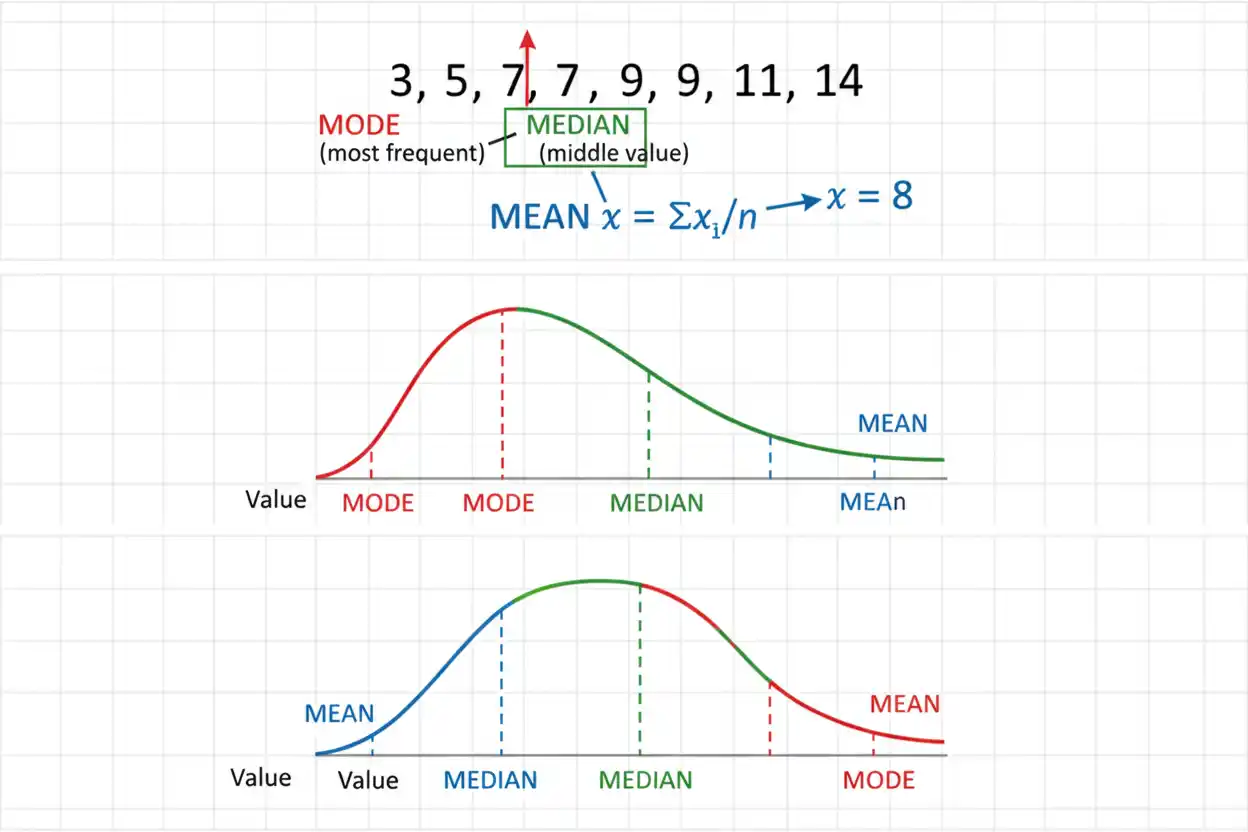
Mean, median, mode are three fundamental measures of central tendency used to describe where numerical or categorical data tend to concentrate. The mean is the arithmetic average obtained by adding numerical observations and dividing by their count, the median is the middle position after values are ordered, and the mode is the value or category occurring most frequently. Although all three can describe a form of center, they respond very differently to skewness, extreme observations, repeated values, and the measurement scale of the data. The mean uses every numerical observation and is therefore highly informative but sensitive to outliers, while the median depends primarily on order and is considerably more resistant to extreme values. The mode depends on frequency rather than numerical distance, making it useful even for nominal categorical data where calculating a mean or median would be meaningless. A symmetric unimodal distribution may have mean, median, mode at approximately the same location, but skewed or irregular data can separate them substantially. Choosing among mean, median, mode therefore requires understanding what each statistic measures rather than treating the three as interchangeable versions of an “average.”
Within core statistics, mean, median, mode provide the principal starting points for describing central tendency. They belong to the broader Statistics & Probability framework, while the arithmetic mean has its own detailed treatment when calculation and properties of that statistic are the main focus.
What Are Mean, Median, Mode?
Mean, median, mode summarize data in three different ways.
The basic distinction is:
Mean = arithmetic balance point
Median = middle ordered position
Mode = most frequent value or category
For example, consider:
2, 3, 3, 5, 7, 10
The mean is:
(2 + 3 + 3 + 5 + 7 + 10)/6
= 30/6
= 5
The median is the average of the two middle values:
(3 + 5)/2
= 4
The mode is:
3
because 3 occurs more often than any other value.
Therefore:
Mean = 5
Median = 4
Mode = 3
The three measures do not have to be equal.
Mean Formula
For numerical observations:
x₁, x₂, …, xₙ
the sample arithmetic mean is:
x̄ = Σxᵢ/n
where:
- x̄ = sample mean
- xᵢ = individual observation
- n = number of observations
- Σ = summation
For a complete finite population:
μ = Σxᵢ/N
where:
- μ = population mean
- N = population size
The mean incorporates every observation directly.
Changing any one numerical value changes the total and therefore changes the mean.
Median Formula
The median must be calculated after arranging observations in ascending or descending order.
For an odd number of ordered observations:
Median position = (n + 1)/2
For example, if:
n = 7
then:
Median position = (7 + 1)/2
= 4
The fourth ordered observation is the median.
For an even number of observations, there are two central values. The median is their arithmetic average:
Median = [x₍ₙ⁄₂₎ + x₍ₙ⁄₂₊₁₎]/2
where the values are ordered.
For:
n = 6
the central positions are:
3 and 4
so:
Median = (3rd value + 4th value)/2
Mode Definition
The mode is the observation or category with the highest frequency.
There is no arithmetic formula comparable to:
x̄ = Σxᵢ/n
Instead, count how often each value or category occurs.
For:
2, 3, 3, 3, 5, 5, 8
the frequencies are:
2 → 1 time
3 → 3 times
5 → 2 times
8 → 1 time
Therefore:
Mode = 3
The mode does not depend on numerical distance between values.
It depends only on frequency.
Mean, Median, Mode Example
Consider:
4, 5, 5, 7, 9, 12, 14
There are seven observations.
Calculate the Mean
Add the values:
4 + 5 + 5 + 7 + 9 + 12 + 14 = 56
Then:
Mean = 56/7
Mean = 8
Find the Median
Because:
n = 7
the median position is:
(7 + 1)/2 = 4
The fourth observation is:
7
Therefore:
Median = 7
Find the Mode
The value 5 occurs twice.
Every other value occurs once.
Therefore:
Mode = 5
The result is:
Mean = 8
Median = 7
Mode = 5
This example shows that mean, median, mode can describe noticeably different locations in the same data set.
Why the Three Measures Differ
Mean, median, mode react to data structure differently.
The mean depends on the numerical magnitude of every observation.
The median depends primarily on rank or position.
The mode depends on frequency.
Suppose the largest value in a data set changes from:
20
to:
2,000
The mean may change dramatically.
The median may not change at all if the observation remains in the same extreme position.
The mode may also remain unchanged unless the frequency pattern changes.
This difference is one of the main reasons analysts choose among mean, median, mode according to the shape and scale of the data.
Mean as an Arithmetic Balance Point
The mean has an important balancing property.
For any sample:
Σ(xᵢ − x̄) = 0
Positive deviations above the mean exactly balance negative deviations below it.
Consider:
2, 4, 6, 8, 10
The mean is:
6
The deviations are:
−4, −2, 0, 2, 4
and:
−4 − 2 + 0 + 2 + 4 = 0
This balance-point interpretation distinguishes the mean from the median and mode.
Median as an Ordered Middle
The median does not attempt to balance numerical deviations.
Instead, it divides ordered observations into lower and upper portions.
For an odd number of observations, approximately half lie below the median and half lie above it.
For example:
1, 4, 7, 9, 15
has median:
7
Two observations lie below 7 and two lie above it.
This positional property makes the median resistant to the exact magnitude of extreme observations.
Mode as a Frequency Peak
The mode identifies the most frequently occurring value.
Suppose:
1, 2, 2, 2, 50, 100
Then:
Mode = 2
The values 50 and 100 have no effect on that result because neither changes the fact that 2 has the highest frequency.
For categorical data, the mode can identify the most common category even when arithmetic calculations are impossible.
For example:
Red, Blue, Blue, Green, Blue, Red
has:
Mode = Blue
There is no meaningful arithmetic mean of those color labels.
Mean, Median, Mode With Odd Sample Size
Consider:
3, 5, 5, 8, 14
The mean is:
(3 + 5 + 5 + 8 + 14)/5
= 35/5
= 7
The median is the third observation:
5
The mode is:
5
Therefore:
Mean = 7
Median = 5
Mode = 5
The relatively large value 14 pulls the mean upward while leaving the median and mode unchanged.
Mean, Median, Mode With Even Sample Size
Consider:
2, 3, 3, 5, 7, 10
The mean is:
30/6
= 5
The two middle observations are:
3 and 5
so:
Median = (3 + 5)/2
= 4
The most frequent value is:
Mode = 3
Therefore:
Mean = 5
Median = 4
Mode = 3
For even n, the median can be a value that does not occur in the original data.
Effect of an Outlier
Consider:
10, 11, 12, 13, 14
The mean is:
12
The median is:
12
There is no unique mode because each value occurs once.
Now replace 14 with 100:
10, 11, 12, 13, 100
The new mean is:
(10 + 11 + 12 + 13 + 100)/5
= 146/5
= 29.2
The median remains:
12
There is still no unique mode.
One extreme value shifts the mean from 12 to 29.2 but does not change the median.
This demonstrates the median’s resistance to extreme magnitudes.
Mean vs Median With Outliers
The mean is sensitive because every observation enters:
Σxᵢ
directly.
The median cares mainly about ordering.
Suppose:
2, 3, 4, 5, 1,000
The mean is:
1,014/5
= 202.8
The median is:
4
Most observations lie between 2 and 5, so the median may better represent the central position of a typical observation.
The mean is still mathematically correct. It represents the total divided equally across all five values.
The appropriate statistic depends on which concept of center matters.
Mean vs Mode With Outliers
Mode is usually unaffected by a single extreme observation unless that value occurs frequently enough to become the most common.
Suppose:
4, 4, 4, 5, 6, 1,000
The mode remains:
4
The mean becomes:
1,023/6
= 170.5
The enormous difference illustrates that mode and mean answer fundamentally different questions.
The mode identifies frequency concentration.
The mean identifies arithmetic balance.
Median vs Mode
Median and mode are both more resistant than the mean to individual extreme magnitudes, but they are not interchangeable.
Consider:
1, 2, 2, 2, 20, 30, 40
The median is:
2
The mode is also:
2
Now consider:
1, 1, 2, 3, 4, 4, 4
The median is:
3
The mode is:
4
The median tracks ordered position.
The mode tracks frequency concentration.
Unimodal Data
A distribution is unimodal when it has one mode.
For example:
1, 2, 3, 3, 3, 4, 5
has:
Mode = 3
A smooth probability distribution can also be unimodal when its density has a single peak.
Many familiar statistical distributions are unimodal.
In a perfectly symmetric unimodal distribution, mean, median, mode can coincide.
Bimodal Data
A data set is bimodal when two values share the highest frequency.
For example:
1, 2, 2, 3, 4, 4, 5
The frequencies of:
2 and 4
are both two.
Every other value occurs once.
Therefore, the data are bimodal with:
Modes = 2 and 4
A bimodal pattern can sometimes indicate that two subpopulations or processes are mixed together.
The cause should be investigated rather than automatically interpreting a single numerical center.
Multimodal Data
A data set with more than two highest-frequency peaks can be described as multimodal.
For example:
1, 1, 2, 2, 3, 3, 4
has three modes:
1, 2, 3
Each occurs twice.
Multimodality can reveal meaningful clustering that the mean and median alone may hide.
A single measure of central tendency is often insufficient when data have several distinct peaks.
Can a Data Set Have No Mode?
Under one common elementary convention, a finite data set in which every value occurs equally often is said to have no mode.
For example:
2, 4, 6, 8
contains four values, each occurring once.
There is no uniquely most frequent observation.
Some definitions may instead say all values tie for maximum frequency, so terminology can vary.
In ordinary descriptive practice, such a data set is usually reported as having no distinct mode.
Mean, Median, Mode in Symmetric Distributions
For a perfectly symmetric unimodal population distribution, mean, median, mode often coincide at the center.
The normal distribution provides the classic example:
Mean = Median = Mode = μ
The normal density is symmetric around μ and has its unique maximum there.
This equality is a useful property of that particular distribution.
It should not be assumed for arbitrary data.
Mean, Median, Mode in Right-Skewed Data
Right-skewed data have a long tail extending toward larger values.
A typical pattern can be:
Mode < Median < Mean
because large values in the right tail pull the arithmetic mean upward.
For example:
1, 2, 2, 3, 4, 10, 30
The mode is:
2
The median is:
3
The mean is:
52/7
≈ 7.43
So:
Mode = 2
Median = 3
Mean ≈ 7.43
The ordering reflects the influence of the right tail.
However, this relationship is a common heuristic, not a universal theorem for every possible right-skewed sample.
Mean, Median, Mode in Left-Skewed Data
Left-skewed data have a longer tail toward smaller values.
A common pattern is:
Mean < Median < Mode
because unusually small observations pull the mean downward.
For example:
−20, 1, 5, 6, 7, 7, 7
The mean is:
13/7
≈ 1.86
The median is:
6
The mode is:
7
Therefore:
Mean ≈ 1.86
Median = 6
Mode = 7
Again, this ordering is a useful descriptive tendency rather than an infallible classification rule.
Why Mean–Median Ordering Is Only a Heuristic
It is tempting to diagnose skewness solely by comparing the mean and median.
For example:
Mean > Median → right skew
is often useful as an informal clue.
However, distribution shape depends on the entire arrangement of observations.
Mixtures, multiple modes, unusual tails, and discrete structures can produce exceptions.
A histogram, density plot, box plot, or quantile analysis provides more direct evidence of distribution shape.
Mean, median, mode should therefore support visual and structural analysis rather than replace it.
Mean, Median, Mode and Measurement Scale
The type of variable determines which measures are meaningful.
Nominal Data
Nominal variables have categories without meaningful ordering.
Examples:
Eye color
Country
Product category
Mode can be meaningful.
Mean and median generally are not.
Ordinal Data
Ordinal categories have a meaningful order but not necessarily equal numerical spacing.
Examples:
Low, Medium, High
Satisfaction ratings
Median and mode can often be meaningful.
An arithmetic mean requires stronger assumptions about the numerical coding.
Interval and Ratio Data
For quantitative variables with meaningful numerical distances, mean, median, mode can all potentially be used.
Which one is most informative depends on the distribution and analytical purpose.
Why the Mean Is Not Suitable for Arbitrary Category Codes
Suppose:
1 = Red
2 = Blue
3 = Green
and the observed codes are:
1, 1, 2, 3
The numerical mean is:
7/4
= 1.75
But:
1.75
has no meaningful color interpretation.
The labels 1, 2, and 3 are identifiers, not measured quantities.
The mode, however, is meaningful:
Red
because Red is the most frequent category.
Median for Ordinal Data
Suppose ordered satisfaction categories are:
Very dissatisfied
Dissatisfied
Neutral
Satisfied
Very satisfied
The median can identify the middle ordered response even if the distances between categories are not assumed equal.
For example, if the ordered responses are:
Dissatisfied, Neutral, Neutral, Satisfied, Very satisfied
the middle response is:
Neutral
This positional interpretation does not require treating the category steps as equal numerical intervals.
Mode for Categorical Data
Mode is the only one of mean, median, mode that can be used naturally with purely nominal categories.
Suppose preferred payment methods are:
Card, Cash, Card, Mobile, Card, Cash
The mode is:
Card
This tells us the most commonly observed category.
Calculating an arithmetic average of category codes would provide no inherent statistical meaning.
Mean and Frequency Tables
When data are summarized by frequencies, the mean can be calculated as:
x̄ = Σfᵢxᵢ/Σfᵢ
where:
- xᵢ = observed value
- fᵢ = frequency
Suppose:
| Value | Frequency |
|---|---|
| 1 | 2 |
| 2 | 5 |
| 3 | 3 |
| 4 | 1 |
The total frequency is:
2 + 5 + 3 + 1 = 11
The weighted total is:
1(2) + 2(5) + 3(3) + 4(1)
= 2 + 10 + 9 + 4
= 25
Therefore:
Mean = 25/11
≈ 2.273
Median From a Frequency Table
Using the same frequency table:
Total n = 11
The median position is:
(11 + 1)/2
= 6
Now accumulate frequencies.
Value 1 occupies positions:
1–2
Value 2 occupies positions:
3–7
Therefore, the sixth observation is:
2
So:
Median = 2
Mode From a Frequency Table
The mode is simply the value with the greatest frequency.
The frequencies are:
1 → 2
2 → 5
3 → 3
4 → 1
The largest frequency is:
5
Therefore:
Mode = 2
For this distribution:
Mean ≈ 2.273
Median = 2
Mode = 2
Weighted Mean Is Different From Median and Mode
A weighted mean allows observations or values to receive unequal numerical weights:
x̄w = Σwᵢxᵢ/Σwᵢ
The median and mode do not automatically use those same weights unless a weighted version of the statistic is explicitly defined.
Therefore, if a data set uses survey weights, probability weights, or exposure weights, the exact definitions of weighted center should be stated.
A weighted arithmetic mean is not directly comparable with an unweighted median unless the analytical objective justifies that comparison.
Mean, Median, Mode and Missing Values
Missing observations are not zeros.
Suppose the observed data are:
4, 6, missing, 10
Replacing the missing observation with zero gives:
Mean = 5
while using the available observed values gives:
Mean = 20/3
≈ 6.67
The median and mode can also change depending on how missing observations are handled.
The correct treatment depends on why data are missing and on the statistical procedure.
Systematic missingness can bias all measures of central tendency.
Mean, Median, Mode and Duplicate Values
Duplicate observations strongly affect the mode and also contribute repeatedly to the mean.
For:
2, 2, 2, 5, 9
the mean is:
20/5
= 4
The median is:
2
The mode is:
2
The repeated value 2 occupies three of the five positions, placing both the median and mode there.
The mean remains higher because the numerical values 5 and 9 contribute to the total.
Mean, Median, Mode and Sample Size
Increasing sample size does not force mean, median, mode to become equal.
Their relationship depends on the underlying distribution.
If samples come from a symmetric unimodal population, larger samples may produce estimates increasingly concentrated near a common population center.
If the population is skewed, the population mean, median, and mode can remain permanently different no matter how large the sample becomes.
More observations improve estimation precision under suitable sampling conditions, but they do not erase genuine differences among central-tendency parameters.
Sample Mean vs Population Mean
The sample arithmetic mean is:
x̄
The population arithmetic mean is:
μ
The sample statistic can estimate the population parameter.
Different random samples generally produce different x̄ values.
The same distinction can be made between a sample median and population median.
A sample mode can also differ from the population’s most probable or most frequent value.
Sampling variability applies to all estimated measures of center.
Mean, Median, Mode and Sampling Variability
Suppose repeated samples are drawn from the same population.
Each sample can produce a different:
- mean,
- median,
- mode.
The sample mean has especially well-developed sampling theory.
The sample median also has a sampling distribution and inferential methods.
The sample mode can be less stable, particularly when frequencies are similar or data are continuous.
Therefore, a measure that is easy to calculate descriptively is not necessarily equally easy to estimate precisely from a limited sample.
Why Mode Can Be Unstable
Suppose frequencies are:
A = 50
B = 49
In the sample:
Mode = A
A small change in only two observations could make:
B
the mode.
By contrast, the arithmetic mean of a large quantitative sample may change only slightly when a few moderate observations are altered.
Mode stability therefore depends heavily on the frequency structure of the population and sample.
Mean, Median, Mode and Continuous Data
In continuous data, exact values may rarely repeat.
For example, accurately measured heights might be:
171.2, 171.8, 172.1, 172.4, 173.0
Every exact value can occur only once.
A raw-data mode may therefore be absent or uninformative.
For a continuous probability distribution, however, mode has a different interpretation: it is the value at which the probability density reaches a maximum.
This distinguishes a theoretical distribution mode from simple repetition counts in finite measurements.
Mean, Median, Mode of the Normal Distribution
For a normal distribution with parameters μ and σ:
Mean = μ
Median = μ
Mode = μ
Therefore:
Mean = Median = Mode
The equality follows from the distribution’s symmetry and its single density peak.
Changing σ changes the spread but does not separate the three measures of center.
This is a special property of the normal model rather than a general rule for probability distributions.
Mean, Median, Mode of Discrete Distributions
Discrete probability distributions can have distinct central measures.
For example, a right-skewed count distribution may have its mode below its mean.
The median may lie between them or coincide with one, depending on the parameters.
A negative binomial distribution, for example, can be substantially right-skewed under some parameter choices, so its mean, median, mode need not coincide.
The exact formulas also depend on the parameterization used.
This reinforces the importance of distinguishing general measures of center from distribution-specific formulas.
Mean and Variance
Mean and variance answer complementary questions.
Mean describes central location.
Variance describes squared dispersion around the mean.
The separate mean and variance topic develops that relationship in detail.
Two distributions can have:
identical mean
but:
different variance.
Similarly, knowing mean, median, mode tells us much about central tendency but not necessarily how broadly the observations are spread.
Measures of center should therefore be paired with appropriate measures of dispersion when a fuller description is needed.
Mean Absolute Deviation
Another spread measure is mean absolute deviation, which commonly calculates:
MAD = Σ|xᵢ − x̄|/n
This measures the average absolute distance from the arithmetic mean.
It differs fundamentally from the median, even though both involve ideas related to absolute distance.
A particularly important mathematical result is:
The arithmetic mean minimizes squared deviations.
The median minimizes absolute deviations.
This difference explains why the mean is central to least-squares methods while the median is naturally connected with absolute-loss optimization.
Mean Minimizes Squared Error
Consider choosing one constant c to represent all observations.
Define squared loss:
L(c) = Σ(xᵢ − c)²
The value that minimizes this quantity is:
c = x̄
the arithmetic mean.
This property is one reason the mean appears throughout least-squares regression and variance calculations.
Large errors are heavily penalized because they are squared.
Median Minimizes Absolute Error
Now define absolute loss:
L(c) = Σ|xᵢ − c|
The value or interval of values minimizing this quantity is a median.
Consider:
0, 0, 0, 10
The mean is:
2.5
Total absolute distance from the mean is:
2.5 + 2.5 + 2.5 + 7.5
= 15
Using the median:
0
gives:
0 + 0 + 0 + 10
= 10
Thus, the median can provide a more resistant center when absolute deviations are the relevant loss measure.
Choosing Mean, Median, Mode
A useful choice depends on the variable and distribution.
Use the Mean When
The mean is often appropriate when:
- data are genuinely quantitative,
- additive differences matter,
- the distribution is reasonably symmetric,
- extreme values are not disproportionately influential,
- total quantities are relevant,
- downstream methods use mean-based models.
Use the Median When
The median is often useful when:
- data are skewed,
- extreme values are present,
- ordinal position matters,
- a robust central location is desired,
- the middle observation has direct substantive meaning.
Use the Mode When
The mode is useful when:
- the most common value matters,
- data are categorical,
- frequency peaks are important,
- a distribution may have one or several prominent clusters.
No single measure is universally superior.
Best Measure for Income Data
Income distributions are often strongly right-skewed.
A small number of very high incomes can pull the arithmetic mean upward.
Therefore, median income is often useful when the question is:
What income lies at the middle of the population?
However, mean income remains meaningful for other questions, such as:
What is total income divided equally per person?
The correct statistic depends on the concept being measured.
Calling one measure “better” without specifying the purpose is incomplete.
Best Measure for Exam Scores
If exam scores are roughly symmetric without severe outliers, the mean can provide a useful summary.
If a few unusual scores distort the distribution, the median can provide additional perspective.
The mode can identify the most frequently achieved exact score, but with a wide score range it may be unstable or less informative.
Reporting both a central measure and a spread measure often provides a clearer view of performance.
Best Measure for Categorical Preferences
Suppose respondents choose:
Product A, Product B, Product C
There is no meaningful numerical mean.
There may also be no inherent order, so the median is undefined.
The mode is appropriate because it identifies the most frequently selected product.
This demonstrates why mode has a role that neither mean nor median can replace.
Mean, Median, Mode and Rounding
Premature rounding can affect the mean.
Suppose:
Mean = 7.4867
Rounding to:
7.49
for reporting may be appropriate.
But if that mean will be used in later calculations, retaining additional precision reduces cumulative rounding error.
Median usually requires less arithmetic, although an even sample can produce a decimal midpoint.
Mode typically requires no rounding unless values themselves have been rounded before frequencies are counted.
Measurement precision can affect apparent modes in continuous data.
How Grouping Can Change the Mode
Suppose exact numerical measurements are almost all unique.
After grouping them into intervals such as:
0–10
10–20
20–30
one interval may clearly have the largest frequency.
That interval can be called the modal class.
However, the modal class is not necessarily the exact mode of the ungrouped observations.
Grouping loses information and can change the apparent frequency structure.
Modal Class
For grouped data, the class interval with the greatest frequency is the modal class.
Suppose:
| Interval | Frequency |
|---|---|
| 0–10 | 4 |
| 10–20 | 9 |
| 20–30 | 6 |
| 30–40 | 2 |
The modal class is:
10–20
because its frequency:
9
is the largest.
This identifies where observations are most concentrated at the grouped level.
It does not imply that every value inside 10–20 occurs equally often.
Median From Grouped Data
For grouped continuous data, the exact median may not be known because individual observations inside each interval are unavailable.
An interpolated grouped-data median can be estimated using cumulative frequencies and the median class.
The result depends on assumptions about how observations are distributed within that class.
Therefore, a median calculated from raw data is exact for those observations, while a grouped-data median may be an approximation.
Mean From Grouped Data
The mean of grouped continuous data is commonly approximated using class midpoints:
Approximate mean = Σfᵢmᵢ/Σfᵢ
where:
- fᵢ = class frequency
- mᵢ = class midpoint
The result is approximate because each observation in a class is represented by the midpoint.
Wider class intervals can produce larger approximation errors.
This contrasts with an exact mean calculated from the original observations.
Mean, Median, Mode and Transformations
Measures of center respond predictably to some transformations.
Suppose:
Y = aX + b
with:
a > 0
Then:
Mean(Y) = aMean(X) + b
Median(Y) = aMedian(X) + b
and modes transform correspondingly when the transformation is one-to-one:
Mode(Y) = aMode(X) + b
For:
a < 0
the ordering reverses, but the transformed median remains the corresponding transformed central value.
Nonlinear transformations can change relationships among mean, median, mode more substantially.
Adding a Constant
Suppose data have:
Mean = 10
Median = 9
Mode = 8
Add:
100
to every value.
The new measures become:
Mean = 110
Median = 109
Mode = 108
The entire distribution shifts without changing its shape.
The differences among the three central measures remain the same.
Multiplying by a Positive Constant
Suppose:
Mean = 5
Median = 4
Mode = 3
Multiply every observation by:
10
Then:
Mean = 50
Median = 40
Mode = 30
The measurement scale changes, but the relative structure remains.
This property is useful when converting units.
Mean, Median, Mode Cannot Describe Spread
Consider:
A: 9, 10, 10, 10, 11
and:
B: −100, 10, 10, 10, 120
Both have:
Median = 10
Mode = 10
Their means are also:
A mean = 10
B mean = 10
Thus:
Mean = Median = Mode = 10
for both data sets.
Yet their spreads are radically different.
This demonstrates why measures such as variance, standard deviation, interquartile range, or absolute deviation are necessary.
Mean, Median, Mode Cannot Fully Describe Shape
Two distributions can also share similar central measures and spread while differing in:
- skewness,
- tail thickness,
- multiple peaks,
- gaps,
- clusters.
A complete statistical description often requires:
- graphical displays,
- quantiles,
- measures of variability,
- context about how data were generated.
Mean, median, mode are foundational summaries, not complete representations of a distribution.
Common Mean, Median, Mode Mistakes
One common error is calculating the median before sorting the data.
The median depends on ordered position.
Another mistake is treating the mode as the largest numerical value rather than the most frequent value.
A third error is assuming the mean must be one of the observations.
It does not.
Another mistake is using the arithmetic mean for nominal category labels merely because categories were assigned numeric codes.
Analysts can also claim that right-skewed data must always satisfy:
Mean > Median > Mode
although that pattern is only a common tendency.
Another error is assuming the median is completely unaffected by every data change. Enough changes in the ordered values can move the median substantially.
It is also incorrect to claim that every data set has exactly one mode.
A sample can be unimodal, bimodal, multimodal, or have no distinct mode.
Finally, no measure of central tendency should be interpreted as a complete description of variability or distribution shape.
How to Calculate Mean, Median, Mode Step by Step
A reliable procedure is:
Step 1: Sort the Data
Ordering is essential for the median and helps reveal repeated values.
Step 2: Calculate the Mean
Mean = Σxᵢ/n
Step 3: Determine Whether n Is Odd or Even
If n is odd:
Median = middle ordered observation
If n is even:
Median = average of the two central observations
Step 4: Count Frequencies
Identify the value or values occurring most frequently.
That gives the mode.
Step 5: Check the Distribution
Look for:
- extreme observations,
- skewness,
- repeated values,
- multiple modes.
Step 6: Choose the Most Informative Measure
Do not automatically report the mean if the median or mode better matches the variable and analytical question.
Full Worked Example
Consider:
1, 3, 3, 4, 6, 7, 8, 24
The data are already ordered.
There are:
n = 8
observations.
Mean
The total is:
1 + 3 + 3 + 4 + 6 + 7 + 8 + 24
= 56
Therefore:
Mean = 56/8
= 7
Median
The central observations are positions 4 and 5:
4 and 6
Therefore:
Median = (4 + 6)/2
= 5
Mode
The value:
3
occurs twice.
Every other value occurs once.
Therefore:
Mode = 3
The result is:
Mean = 7
Median = 5
Mode = 3
The relatively large value 24 pulls the arithmetic mean upward, while the median and mode remain closer to the main cluster of observations.
How to Report Mean, Median, Mode
A concise descriptive report might state:
Mean = 7, median = 5, mode = 3.
If skewness or extreme observations matter, add interpretation:
The mean exceeds the median because the high observation at 24 pulls the arithmetic average upward.
For categorical data, report the mode using the category label rather than an arbitrary numeric code.
When comparing groups, use the same definitions and measurement scale consistently.
Frequently Asked Questions About Mean, Median, Mode
What are mean, median, mode?
Mean, median, mode are measures of central tendency. The mean is the arithmetic average, the median is the middle ordered value, and the mode is the most frequent value or category.
What is the formula for the mean?
For a sample:
x̄ = Σxᵢ/n
How do you calculate the median?
Sort the data first. For odd n, choose the middle observation. For even n, average the two middle observations.
How do you calculate the mode?
Count the frequency of every value or category. The one with the greatest frequency is the mode.
Can mean, median, mode be equal?
Yes. In some symmetric unimodal distributions, including the normal distribution:
Mean = Median = Mode
Can mean, median, mode all be different?
Yes. Skewed or irregular data frequently produce different values for all three.
Is the mean the same as average?
In basic numerical statistics, “average” commonly means arithmetic mean, although average can be used more broadly in everyday language.
Is the median affected by outliers?
It is much less sensitive to extreme magnitudes than the mean, although changes affecting central ordered positions can alter it.
Is the mean affected by outliers?
Yes. Every observation contributes to the total, so extreme values can strongly influence the mean.
Is the mode affected by outliers?
An isolated extreme value usually does not affect the mode unless it changes the highest-frequency value.
Can the mean be a value that does not appear in the data?
Yes.
Can the median be a value that does not appear in the data?
Yes. With an even number of observations, the median can be the average of two central values and may not itself be observed.
Can the mode be a value that does not appear in the data?
No. For a finite raw data set, the mode must be one of the observed values or categories.
Can there be two modes?
Yes. A data set with two equally most frequent values is bimodal.
Can there be more than two modes?
Yes. Several values can tie for the highest frequency, producing a multimodal data set.
Can there be no mode?
Yes, under the common convention that a distinct mode requires one or more values to occur more frequently than the others.
Which measure is best for skewed data?
The median is often useful because it is resistant to extreme tails, but the appropriate measure depends on the question being answered.
Which measure is best for categorical data?
For nominal categories, the mode is the natural measure of central frequency. Mean and median may not be meaningful.
Which measure is best for symmetric numerical data?
The mean is often highly informative when the distribution is reasonably symmetric and free from influential extreme observations.
Why is the median resistant to outliers?
It depends primarily on ordered position rather than the exact numerical magnitude of extreme values.
Does the mean minimize squared error?
Yes. The arithmetic mean minimizes:
Σ(xᵢ − c)²
over choices of c.
Does the median minimize absolute error?
Yes. A median minimizes:
Σ|xᵢ − c|
over choices of c.
What is the relationship between mean, median, mode and skewness?
Right-skewed data often have the mean pulled to the right of the median and mode, while left-skewed data often show the reverse. These patterns are useful heuristics rather than universal rules.
What are mean, median, mode for a normal distribution?
For a normal distribution:
Mean = Median = Mode = μ
Is mode useful for continuous data?
Exact repeated observations may be rare in raw continuous measurements, but a continuous probability distribution can have a mode defined by the maximum of its density.
Why should mean, median, mode be reported with a spread measure?
Measures of central tendency describe location but not dispersion. Two data sets can have identical centers while having completely different variability.
What is the difference between mean and mean absolute deviation?
The mean describes center. Mean absolute deviation describes the average absolute distance of observations from a center, commonly the arithmetic mean.
What is the difference between mean and variance?
Mean describes arithmetic center. Variance describes squared dispersion around the mean.
Can two distributions have the same mean, median, mode?
Yes. They can still differ substantially in variance, tails, skewness, or other structural features.
Should the mean always be preferred because it uses every value?
No. Using every value makes the mean informative but also makes it sensitive to extreme observations. The appropriate measure depends on the data and the intended interpretation.




