


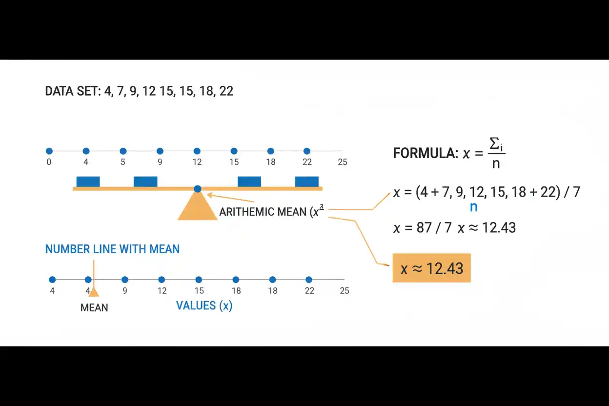
The mean is one of the most widely used measures of central tendency in statistics. It summarizes a collection of numerical values by adding them together and dividing by the number of observations, producing a single value that represents the arithmetic average of the data. For sample data, the arithmetic mean is commonly written as x̄, while the population mean is usually represented by μ. The mean uses every numerical observation in the data set, which makes it highly informative but also sensitive to unusually large or small values. It is especially useful when the data are quantitative, the center of the distribution is meaningful, and extreme observations do not distort the summary beyond what the analysis can tolerate. The mean also appears throughout probability, estimation, regression, variability calculations, and many other statistical methods. However, it should not automatically be treated as the “typical” value for every distribution, particularly when data are strongly skewed or contain influential outliers.
The mean is a foundational concept within core statistics and the broader Statistics & Probability framework. It acts as a central reference point for many statistical calculations while remaining distinct from measures of spread such as the interquartile range and from specialist topics that combine mean and variance in a broader distributional context.
What Is the Mean?
The arithmetic mean is calculated by summing all numerical observations and dividing by the number of observations.
For values:
x₁, x₂, x₃, …, xₙ
the sample mean is:
x̄ = Σxᵢ/n
where:
- x̄ = sample mean
- Σ = sum
- xᵢ = individual sample observation
- n = number of sample observations
For example, consider:
4, 6, 8, 10, 12
Add the values:
4 + 6 + 8 + 10 + 12 = 40
There are:
n = 5
observations.
Therefore:
x̄ = 40/5
x̄ = 8
The arithmetic average of the data is:
8
Mean Formula
The standard sample formula is:
x̄ = Σxᵢ/n
The corresponding finite-population formula is:
μ = Σxᵢ/N
where:
- μ = population mean
- N = number of population observations
The arithmetic operation is structurally the same.
The distinction lies in what the observations represent.
If every member of the population of interest is included, the result is a population parameter:
μ
If the observations form a sample used to learn about a larger population, the result is a sample statistic:
x̄
This population-versus-sample distinction is important throughout statistical inference.
What Does the Mean Represent?
The mean can be interpreted as the equal-share value of a data set.
Suppose five people have quantities:
2, 4, 6, 8, 10
The total is:
30
If that total were redistributed equally among all five observations:
30/5 = 6
Each would have:
6
That equal-share interpretation is the arithmetic mean.
It helps explain why the mean depends on the total sum of the values rather than merely their positions in an ordered list.
Mean as a Balance Point
The mean also acts as a numerical balance point.
For data:
2, 4, 6, 8, 10
the mean is:
6
Calculate deviations from 6:
2 − 6 = −4
4 − 6 = −2
6 − 6 = 0
8 − 6 = 2
10 − 6 = 4
Add those deviations:
−4 − 2 + 0 + 2 + 4 = 0
This is not a coincidence.
For any numerical sample:
Σ(xᵢ − x̄) = 0
The positive and negative deviations from the sample mean always balance exactly.
Why Deviations From the Mean Sum to Zero
Start with:
Σ(xᵢ − x̄)
Distribute the sum:
Σxᵢ − Σx̄
Because x̄ is the same constant for all n observations:
Σx̄ = nx̄
Therefore:
Σ(xᵢ − x̄) = Σxᵢ − nx̄
But:
x̄ = Σxᵢ/n
so:
nx̄ = Σxᵢ
Therefore:
Σ(xᵢ − x̄) = 0
This identity is fundamental to many statistical formulas involving deviations, variance, covariance, and regression.
Mean Example
Consider the data:
7, 9, 10, 14, 15
First calculate the sum:
7 + 9 + 10 + 14 + 15 = 55
The number of observations is:
n = 5
Therefore:
x̄ = 55/5
x̄ = 11
The sample mean is:
11
Notice that 11 does not appear in the original data.
A mean does not have to equal one of the observed values.
It is a calculated center, not necessarily an actual observation.
Mean With Decimal Values
The same formula applies to decimals.
Suppose:
2.4, 3.1, 4.7, 5.8
The sum is:
2.4 + 3.1 + 4.7 + 5.8 = 16.0
There are:
n = 4
values.
Therefore:
x̄ = 16/4
x̄ = 4
The result can be an integer even when none of the observations is an integer.
Likewise, integer observations can produce a decimal mean.
Mean With Negative Values
Negative observations do not change the calculation method.
Consider:
−6, −2, 3, 5
The sum is:
−6 − 2 + 3 + 5 = 0
Therefore:
x̄ = 0/4
x̄ = 0
The mean can lie between negative and positive observations.
It can also be negative when the negative total outweighs the positive total.
Mean With Repeated Values
Repeated observations are included every time they occur.
Suppose:
2, 2, 2, 5, 9
The sum is:
20
so:
x̄ = 20/5
x̄ = 4
The value 2 appears three times, so it contributes three times to the total.
Ignoring repeated observations would change both the total and the sample size and therefore produce an incorrect mean.
Mean vs Average
In everyday language, “mean” and “average” are often used interchangeably.
When someone says:
average = sum of values / number of values
they are referring to the arithmetic mean.
However, the word “average” can be used informally for several different measures of center, including the median or mode.
In formal statistical work, saying arithmetic mean is more precise when the calculation is:
Σxᵢ/n
Thus:
Arithmetic mean = a specific mathematical statistic
while:
Average = a broader everyday term that often, but not always, means arithmetic mean
Sample Mean vs Population Mean
Suppose a classroom contains exactly 30 students and the heights of all 30 are measured.
If those 30 students are the complete population of interest, the resulting average height is a population mean:
μ
Now suppose only 10 students are randomly selected from those 30.
The average height of those 10 students is a sample mean:
x̄
The sample mean can be used to estimate the population mean.
However:
x̄
will generally not equal:
μ
exactly because different samples contain different observations.
That difference is sampling variation.
The Sample Mean as an Estimator
One of the most important uses of the sample mean is estimating an unknown population mean.
Suppose the target population has unknown mean:
μ
A random sample is collected and produces:
x̄ = 52.4
Then:
52.4
is the point estimate of μ.
Another random sample from the same population may produce:
x̄ = 51.8
or:
x̄ = 53.1
The estimate varies from sample to sample.
Statistical inference builds on this variation to quantify uncertainty around the population parameter.
Why the Mean Uses Every Observation
The arithmetic mean depends on:
Σxᵢ
Every observation contributes to that sum.
If any value changes while all others remain fixed, the mean changes.
Suppose:
2, 4, 6, 8
The mean is:
5
Change the last observation from 8 to 20:
2, 4, 6, 20
The new mean is:
32/4
= 8
The change in one observation moves the center substantially.
This sensitivity is both a strength and a limitation.
The mean uses all available numerical information, but extreme values can have substantial influence.
Effect of an Outlier on the Mean
Consider:
10, 11, 12, 13, 14
The mean is:
60/5
= 12
Now replace 14 with 100:
10, 11, 12, 13, 100
The sum becomes:
146
so:
x̄ = 146/5
x̄ = 29.2
One unusually large observation shifts the mean from:
12
to:
29.2
even though four of the five observations still lie between 10 and 13.
This is why the mean may not represent a typical observation well in a strongly skewed or outlier-heavy data set.
Mean and the Interquartile Range
The mean describes center.
The interquartile range describes the spread of the middle 50% of ordered observations.
These statistics respond differently to extreme values.
The mean uses every numerical value.
The interquartile range depends mainly on:
Q₁
and:
Q₃
Therefore, a large outlier can move the mean dramatically while leaving the interquartile range unchanged.
For skewed data, it is often useful to examine a robust measure of center and spread alongside or instead of mean-based summaries.
Mean in Symmetric Data
For a reasonably symmetric, unimodal distribution without severe outliers, the mean often provides an informative measure of center.
In a perfectly symmetric population distribution around a central value c, the population mean frequently lies at that center when the mean exists.
For example, a symmetric distribution centered at:
50
may have:
μ = 50
Values above and below the center balance in the expected-value calculation.
This is one reason the mean is particularly natural in many approximately symmetric models.
Mean in Skewed Data
The mean is pulled toward long tails.
Suppose most incomes in a sample lie between:
30,000 and 70,000
but a few observations exceed:
1,000,000
The arithmetic mean can be much larger than what most individuals experience.
That does not make the mean mathematically wrong.
It means the total amount divided equally across observations differs from the center represented by the typical ordered position.
The choice of summary should match the question.
If total economic resources per person matter, the mean can be highly relevant.
If a typical individual’s position is the focus, another center may communicate the distribution differently.
Weighted Mean
Not every observation or category needs to receive equal weight.
A weighted mean has the form:
x̄w = Σwᵢxᵢ / Σwᵢ
where:
- xᵢ = value
- wᵢ = weight attached to that value
If all weights are equal, the weighted mean reduces to the ordinary arithmetic mean.
Suppose course grades are:
Exam = 80 with weight 0.60
Project = 90 with weight 0.30
Participation = 100 with weight 0.10
The weighted mean is:
x̄w = (0.60)(80) + (0.30)(90) + (0.10)(100)
x̄w = 48 + 27 + 10
x̄w = 85
Because the weights sum to 1, no additional division is required in this example.
Weighted Mean When Weights Do Not Sum to One
Suppose:
x₁ = 10 with weight 2
x₂ = 20 with weight 3
x₃ = 40 with weight 5
Then:
Σwᵢxᵢ = 2(10) + 3(20) + 5(40)
= 20 + 60 + 200
= 280
The total weight is:
2 + 3 + 5 = 10
Therefore:
x̄w = 280/10
x̄w = 28
The larger weight attached to 40 pulls the weighted average upward.
Mean From a Frequency Table
A frequency table can be treated as a weighted calculation.
Suppose:
| Value x | Frequency f |
|---|---|
| 2 | 3 |
| 4 | 2 |
| 7 | 5 |
The total frequency is:
Σf = 3 + 2 + 5
= 10
The weighted total is:
Σfx = 3(2) + 2(4) + 5(7)
= 6 + 8 + 35
= 49
Therefore:
x̄ = Σfx/Σf
x̄ = 49/10
x̄ = 4.9
This produces the same result as writing every individual observation out separately.
Mean of Combined Groups
Suppose two groups have different sample sizes.
Group A:
n₁ = 20
x̄₁ = 50
Group B:
n₂ = 30
x̄₂ = 70
The combined mean is not simply:
(50 + 70)/2 = 60
because the group sizes differ.
Instead, recover the totals:
Group A total = 20 × 50 = 1,000
Group B total = 30 × 70 = 2,100
Combined total:
1,000 + 2,100 = 3,100
Combined sample size:
20 + 30 = 50
Therefore:
Combined mean = 3,100/50
= 62
The correct combined value is:
62
The group with more observations receives more weight.
General Combined Mean Formula
For groups indexed by j:
Combined mean = Σnⱼx̄ⱼ / Σnⱼ
where:
- nⱼ = number of observations in group j
- x̄ⱼ = mean of group j
This is another weighted mean.
The weights are the group sample sizes.
Averaging group means equally is correct only when all groups have the same number of observations.
Mean After Adding a Constant
Suppose every observation is increased by the same constant c.
Define:
yᵢ = xᵢ + c
Then:
ȳ = x̄ + c
For example, start with:
2, 4, 6
whose mean is:
4
Add 10 to every value:
12, 14, 16
The new mean is:
14
which equals:
4 + 10
Adding a constant shifts the entire data set and its mean by exactly the same amount.
Mean After Multiplying by a Constant
Suppose:
yᵢ = axᵢ
Then:
ȳ = ax̄
For example:
3, 5, 7
has mean:
5
Multiply every observation by 4:
12, 20, 28
The new mean is:
20
which equals:
4 × 5
This property makes unit conversions straightforward.
If all measurements are converted from meters to centimeters by multiplying by 100, the mean is also multiplied by 100.
General Linear Transformation of the Mean
For:
Y = aX + b
the mean transforms as:
Mean(Y) = aMean(X) + b
In sample notation:
ȳ = ax̄ + b
In population notation:
μY = aμX + b
This linearity property is fundamental.
It also helps explain why the mean appears naturally in linear regression and other linear statistical methods.
Mean and Linear Regression
In ordinary simple linear regression with an intercept, the fitted line passes through:
(x̄, ȳ)
The intercept formula is:
b₀ = ȳ − b₁x̄
Therefore, substituting x̄ into the fitted equation:
ŷ = b₀ + b₁x̄
gives:
ŷ = ȳ
This makes the sample mean central to the geometry of linear regression.
The regression model builds on the mean-only baseline by explaining how expected response values change with predictors.
Mean and Logarithmic Regression
A logarithmic regression model can be fitted by defining:
z = ln(x)
and estimating:
y = a + bz
The intercept can be calculated from:
a = ȳ − bz̄
where:
z̄ = mean of ln(x)
Again, the arithmetic mean appears directly in the regression calculations.
However, the mean of the logarithms:
mean[ln(x)]
is not generally equal to:
ln(mean[x])
That distinction matters whenever nonlinear transformations are involved.
Mean of a Transformed Variable
For a linear transformation:
E(aX + b) = aE(X) + b
But for a nonlinear function g:
E[g(X)]
is generally not equal to:
g[E(X)]
For example:
E(X²) ≠ [E(X)]²
in general.
Likewise:
E[ln(X)] ≠ ln[E(X)]
in general.
This is why transformed-data analyses must calculate the relevant transformed values rather than simply transform the original mean.
Mean and Mean Absolute Deviation
The mean absolute deviation measures average absolute distance from a chosen center, commonly the arithmetic mean in one standard definition.
If deviations from x̄ are:
xᵢ − x̄
then absolute deviations are:
|xᵢ − x̄|
The mean absolute deviation about the arithmetic mean is:
MAD = Σ|xᵢ − x̄|/n
The arithmetic mean therefore serves as the central reference point, while MAD answers a separate question about typical absolute dispersion around that center.
Why Absolute Deviations Do Not Sum to Zero
Raw deviations from x̄ satisfy:
Σ(xᵢ − x̄) = 0
But absolute deviations satisfy:
|xᵢ − x̄| ≥ 0
Therefore, they do not cancel.
For data:
2, 4, 6
the mean is:
4
Raw deviations are:
−2, 0, 2
which sum to zero.
Absolute deviations are:
2, 0, 2
which sum to:
4
This difference is why dispersion measures use absolute values or squared deviations rather than simply averaging signed deviations.
Mean and Variability
A mean describes where data are centered.
It does not describe how tightly observations cluster around that center.
Consider:
Data A: 9, 10, 11
The mean is:
10
Now consider:
Data B: 0, 10, 20
Its mean is also:
10
The two data sets have identical arithmetic centers but very different spread.
Therefore, a mean should often be accompanied by an appropriate variability measure.
The separate topic of mean and variance examines these two distributional quantities together in greater depth.
Same Mean, Different Distributions
Even more dramatically, very different distributions can share the same mean.
Consider:
A = 5, 5, 5, 5, 5
and:
B = −100, 5, 5, 5, 110
Both have total:
25
and therefore:
mean = 5
Yet their statistical structures are radically different.
One has no variation.
The other contains extreme values.
This illustrates why the arithmetic mean cannot summarize an entire distribution by itself.
Mean and Data Units
The arithmetic mean has the same units as the observations.
If values are measured in:
kilograms
then the mean is in kilograms.
If measurements are:
seconds
the mean is in seconds.
If values are:
dollars
the mean is in dollars.
This makes the arithmetic mean directly interpretable on the original measurement scale.
Can the Mean Be Outside the Data Range?
For a nonempty finite set of ordinary real-valued observations with equal positive weights, the arithmetic mean must lie between the minimum and maximum.
Therefore:
Minimum ≤ x̄ ≤ Maximum
If all observations are identical, then:
Minimum = x̄ = Maximum
For positive weighted means, the result likewise lies between the smallest and largest values receiving positive weight.
If a supposed ordinary arithmetic mean lies outside the observed range, the calculation should be checked.
Can the Mean Equal the Minimum or Maximum?
Yes, but only under restrictive conditions for an ordinary unweighted mean.
Suppose all observations are at least:
m
If the mean equals the minimum m, then every observation must equal m.
Likewise, if the mean equals the maximum, all observations must equal that maximum.
For example:
7, 7, 7
has:
minimum = mean = maximum = 7
If any observation were larger than 7, the mean would become larger than the minimum.
Mean of Zero
A data set can have:
x̄ = 0
without every value being zero.
For example:
−3, −1, 1, 3
has total:
0
so:
x̄ = 0
Positive and negative values balance.
Therefore, a zero arithmetic mean should not automatically be interpreted as “no data,” “no effect,” or “all values equal zero.”
Its meaning depends on the measurement scale and context.
Missing Values Are Not Zero
A missing observation should not automatically be entered as:
0
unless zero is the actual observed value.
Suppose the recorded values are:
10, 20, missing
If the missing value is incorrectly replaced with zero:
x̄ = (10 + 20 + 0)/3
= 10
If the available-data average uses only the two observed values:
x̄ = (10 + 20)/2
= 15
Those are very different results.
How missing data should be handled depends on why the observation is missing and on the statistical objective.
Mean With Grouped Continuous Data
When only grouped intervals and their frequencies are available, an approximate mean can be calculated using class midpoints.
Suppose:
| Interval | Midpoint m | Frequency f |
|---|---|---|
| 0–10 | 5 | 4 |
| 10–20 | 15 | 6 |
| 20–30 | 25 | 2 |
Approximate total:
Σfm = 4(5) + 6(15) + 2(25)
= 20 + 90 + 50
= 160
Total frequency:
Σf = 12
Therefore:
Approximate mean = 160/12
≈ 13.33
The word approximate matters because the original individual values within each class are unknown.
Replacing every value by its class midpoint loses information.
Mean of Percentages
Percentages should not always be averaged directly.
Suppose one group has:
90% success among 10 observations
and another has:
50% success among 100 observations
The simple average of the percentages is:
(90% + 50%)/2
= 70%
But the combined success rate is weighted by group size.
Successes:
0.90(10) = 9
0.50(100) = 50
Total successes:
59
Total observations:
110
Combined rate:
59/110
≈ 53.64%
The correct aggregate depends on the denominators.
A simple arithmetic mean of percentages is appropriate only when equal weighting is justified.
Mean of Rates
Rates can present similar problems.
Suppose the average speed over two equal time intervals is being calculated.
The arithmetic mean of the two speeds can be appropriate because the intervals receive equal time weight.
But if the two speeds apply over equal distances, the average speed is not generally the arithmetic mean.
The correct calculation depends on:
total distance / total time
This illustrates a broader principle:
The arithmetic mean is appropriate when the averaging structure matches equal additive contributions.
The word “average” alone does not determine the correct formula.
Arithmetic Mean vs Weighted Mean
The ordinary arithmetic mean gives every observation equal weight:
x̄ = (x₁ + x₂ + … + xₙ)/n
A weighted mean gives different observations different influence:
x̄w = Σwᵢxᵢ/Σwᵢ
The unweighted mean is therefore a special case where:
w₁ = w₂ = … = wₙ
Choosing weights changes the estimand.
Weights should reflect the statistical design, frequency structure, or substantive objective rather than being selected merely to produce a preferred result.
Arithmetic Mean vs Geometric Mean
The arithmetic mean is based on addition:
x̄ = Σxᵢ/n
The geometric mean is based on multiplication and nth roots.
For positive values:
GM = (x₁x₂…xₙ)¹⁄ⁿ
The geometric mean can be useful for multiplicative growth factors, ratios, and compounded changes.
For example, averaging annual growth factors may require a geometric rather than arithmetic interpretation.
However, unless otherwise specified, “mean” in basic descriptive statistics normally refers to the arithmetic mean.
Arithmetic Mean vs Harmonic Mean
For positive nonzero values, the harmonic mean is:
HM = n / Σ(1/xᵢ)
It can be useful for certain rate problems where the denominator structure matters.
The arithmetic, geometric, and harmonic means answer different averaging questions.
For positive values:
HM ≤ GM ≤ AM
under standard conditions, where AM is the arithmetic mean.
The arithmetic mean remains the central focus when observations are combined additively with equal weight.
Mean and Probability Distributions
A probability distribution can also have a theoretical mean.
For a discrete random variable X:
E(X) = ΣxP(X = x)
when the expectation exists.
For a continuous random variable with density f(x):
E(X) = ∫xf(x) dx
when the integral exists.
This theoretical quantity represents a probability-weighted average over the possible values of the random variable.
In probability notation, the terms:
expected value
and:
population mean
are closely connected.
The exact formula depends on whether the distribution is discrete or continuous.
Mean Does Not Always Exist
Not every probability distribution has a finite arithmetic mean.
Some heavy-tailed distributions have no finite expected value.
For example, the theoretical expectation can fail to converge even though individual observations themselves are finite.
This shows that the concept of a mean depends not only on the formula but also on whether the relevant sum or integral is mathematically well defined.
For ordinary finite data sets, by contrast, the arithmetic mean always exists as long as all included values are finite real numbers.
Expected Sample Mean
If observations:
X₁, X₂, …, Xₙ
are drawn from a population with finite mean μ, then:
E(x̄) = μ
under the standard setup.
This means the sample mean is an unbiased estimator of the population mean.
Across repeated samples, the average of the sample means equals the population mean.
An individual sample mean can still be above or below μ.
Unbiasedness is a long-run property of the estimator, not a guarantee for any single sample.
Standard Error of the Sample Mean
If independent observations have population standard deviation σ, the standard error of the sample mean is:
SE(x̄) = σ/√n
When σ is unknown, it is commonly estimated by:
SE(x̄) ≈ s/√n
under suitable conditions.
This formula shows that larger samples usually make the sample mean more precise.
As:
n
increases, the denominator:
√n
increases, reducing the standard error.
This does not mean larger samples eliminate bias from poor sampling methods.
They primarily reduce sampling variability under the model.
Mean and the Central Limit Effect
Under broad conditions, the sampling distribution of the sample mean becomes increasingly close to a normal distribution as sample size grows, even when the original observations are not themselves normally distributed.
This is a central reason the sample mean plays such a major role in statistical inference.
However, the approximation can be slower when distributions are extremely skewed, heavy-tailed, or dominated by unusual observations.
Dependence between observations can also change the standard sampling behavior.
Large n is useful, but it does not automatically repair every violation of a statistical model.
Mean and Sample Size
Suppose a sample contains n observations with mean x̄.
The total can be recovered from:
Σxᵢ = nx̄
For example, if:
n = 25
and:
x̄ = 18
then:
Σxᵢ = 25 × 18
= 450
This identity is useful when combining groups or updating means.
The arithmetic mean stores information about the total relative to the number of observations.
Updating a Mean After Adding One Observation
Suppose the current sample has:
n observations
with mean:
x̄old
The current total is:
nx̄old
Now add a new value:
xnew
The new mean is:
x̄new = (nx̄old + xnew)/(n + 1)
For example, suppose:
n = 4
x̄old = 10
so the current total is:
40
Add:
xnew = 20
Then:
x̄new = (40 + 20)/5
= 12
This allows the mean to be updated without reconstructing every original observation.
Updating a Mean After Removing One Observation
Suppose a sample contains:
n
observations with mean:
x̄old
and one observation xremoved is removed.
The new mean is:
x̄new = (nx̄old − xremoved)/(n − 1)
provided:
n > 1
For example:
n = 5
x̄old = 12
so the total is:
60
Remove:
20
The new mean is:
(60 − 20)/4
= 10
Again, the total-sample relationship makes the update straightforward.
Effect of Changing One Observation
Suppose one observation changes from:
xold
to:
xnew
while n remains constant.
The total changes by:
xnew − xold
Therefore, the mean changes by:
(xnew − xold)/n
For example, with:
n = 10
changing one value from:
20
to:
30
raises the mean by:
(30 − 20)/10
= 1
This shows quantitatively why a single extreme value has less effect in a very large sample than in a very small one, although extremely large changes can still matter.
Why the Mean Minimizes Squared Distance
The arithmetic mean has an important optimization property.
For any constant c, consider:
Σ(xᵢ − c)²
The value of c that minimizes this total squared distance is:
c = x̄
This property explains why the arithmetic mean appears naturally in least-squares methods.
It also helps connect the mean to linear regression, where squared residuals are minimized.
By contrast, minimizing total absolute distance leads to a different measure of center.
Mean and Squared Error
Suppose a single constant must be used to predict every observation.
If prediction error is measured through squared loss:
Loss(c) = Σ(xᵢ − c)²
then the best constant is:
c = x̄
For example, for:
2, 4, 9
the mean is:
5
Using 5 minimizes the sum of squared prediction errors compared with any other constant.
This makes the arithmetic mean especially natural in statistical models built around squared-error loss.
When the Mean Is a Good Summary
The mean is especially informative when:
- observations are quantitative,
- total quantities matter,
- the distribution is reasonably symmetric,
- extreme observations are not unduly dominant,
- additive differences are meaningful,
- downstream statistical methods use mean-based modeling.
It is also valuable when the analysis needs a statistic that incorporates every observation.
A mean should be chosen because it answers the relevant question, not merely because it is the most familiar average.
When the Mean Can Be Misleading
The arithmetic mean can be difficult to interpret when:
- the distribution is strongly skewed,
- a few extreme values dominate the total,
- the variable is ordinal rather than genuinely numerical,
- rates have unequal denominators,
- percentages refer to unequal group sizes,
- nonlinear transformations define the relevant averaging structure,
- the population mean does not exist mathematically.
In those situations, another summary or a more careful weighted calculation may better match the objective.
Mean of Categorical Data
An arithmetic mean is not meaningful for arbitrary category labels.
Suppose categories are coded:
1 = red
2 = blue
3 = green
A mean code of:
1.8
has no inherent color interpretation.
The numerical labels are identifiers rather than measured quantities.
However, binary indicator variables can be different.
If:
X = 1 for success
and:
X = 0 for failure
then:
x̄
equals the sample proportion of successes.
That interpretation is meaningful because the numerical coding has a defined mathematical structure.
Mean of a Binary Variable
Suppose:
Xᵢ ∈ {0,1}
Then:
x̄ = Σxᵢ/n
Since the sum of the 1s equals the number of successes x:
x̄ = x/n
Therefore:
x̄ = p̂
the sample proportion.
For example:
1, 0, 1, 1, 0
has:
x̄ = 3/5
= 0.60
Thus, 60% of the observations are coded as success.
This is an important connection between averages and proportions.
Mean and Rounding
Rounding too early can change the final result.
Suppose the exact intermediate sum gives:
x̄ = 6.3748
If the analysis later requires additional calculations, using:
6.37
too early can introduce avoidable error.
A better approach is to preserve additional precision during intermediate calculations and round the final reported result appropriately.
The number of decimal places should reflect the measurement scale and analytical purpose rather than being selected mechanically.
Common Mean Mistakes
A common mistake is dividing by the wrong number of observations.
For:
n
values, the arithmetic mean is:
Σxᵢ/n
Another error is forgetting repeated observations when calculating the total or sample size.
A third mistake is averaging group means without considering unequal group sizes.
It is also incorrect to treat missing values as zeros unless zero is actually observed.
Another frequent error is averaging percentages with unequal denominators as though all groups had equal weight.
The arithmetic mean can also be misleading when one extreme value dominates a small data set.
Finally, “average” should not automatically be assumed to mean arithmetic mean when the underlying problem involves rates, multiplicative growth, or another specialized averaging structure.
How to Calculate the Mean Step by Step
A reliable calculation is straightforward.
Step 1: Identify the Numerical Observations
List the values to be included.
Step 2: Count the Observations
Determine:
n
for a sample or:
N
for a complete finite population.
Step 3: Add the Values
Calculate:
Σxᵢ
Step 4: Divide by the Count
For a sample:
x̄ = Σxᵢ/n
For a population:
μ = Σxᵢ/N
Step 5: Check the Result
For an ordinary unweighted finite data set:
Minimum ≤ mean ≤ Maximum
Step 6: Add Units
Report the result using the original measurement units.
Step 7: Consider the Distribution
Check whether outliers, skewness, weighting, missing data, or unusual measurement structure make the arithmetic mean difficult to interpret.
Full Worked Example
Suppose ten measurements are:
12, 15, 18, 18, 20, 22, 23, 24, 26, 32
First, calculate the sum:
12 + 15 + 18 + 18 + 20 + 22 + 23 + 24 + 26 + 32
= 210
The sample size is:
n = 10
Therefore:
x̄ = 210/10
x̄ = 21
The sample mean is:
21
Check the range:
Minimum = 12
Maximum = 32
and:
12 ≤ 21 ≤ 32
so the result satisfies the basic range check.
The arithmetic mean tells us that the observations average 21 units when their total is distributed evenly across the ten measurements.
How to Report the Mean
A clear statistical statement identifies the variable, value, and units.
For example:
The sample mean was 21 minutes.
or:
Average measured mass, x̄ = 42.6 g.
If the sample is being used for inference about a larger population, it can also be useful to report:
- sample size,
- standard deviation or another spread measure,
- confidence interval when appropriate.
A mean alone describes center but not uncertainty or variability.
Frequently Asked Questions About the Mean
What is the mean?
The mean is the arithmetic average obtained by adding numerical values and dividing by the number of observations.
What is the mean formula?
For a sample:
x̄ = Σxᵢ/n
For a finite population:
μ = Σxᵢ/N
Is mean the same as average?
In basic statistical usage, “average” often refers to the arithmetic mean. However, average is an informal broader term and can sometimes refer to other measures of center.
How do you calculate the mean?
Add all included numerical values and divide by the number of observations.
What does x̄ mean?
x̄ represents the arithmetic mean of a sample.
What does μ mean?
μ commonly represents a population mean.
Does the mean have to be one of the observations?
No. The arithmetic mean can fall between observed values.
Can the mean be a decimal?
Yes. Integer observations can produce a decimal mean, and decimal observations can produce either decimal or integer means.
Can the mean be negative?
Yes. If the total of the observations is negative, the mean is negative.
Can the mean equal zero?
Yes. Positive and negative values can balance so their sum and therefore their mean equal zero.
Can the mean lie outside the minimum and maximum?
Not for an ordinary finite arithmetic mean with equal positive weights. It must lie between the smallest and largest observations.
Why do deviations from the mean sum to zero?
Because:
Σ(xᵢ − x̄) = Σxᵢ − nx̄ = 0
by the definition of x̄.
Is the mean affected by outliers?
Yes. Because every value contributes directly to the total, extreme observations can move the arithmetic mean substantially.
Is the mean good for skewed data?
It can still be mathematically meaningful, especially when totals matter, but it may not represent a typical observation well when the distribution is strongly skewed.
What is a weighted mean?
A weighted mean gives observations different levels of influence:
x̄w = Σwᵢxᵢ/Σwᵢ
How do you find the mean from a frequency table?
Use frequency as the weight:
x̄ = Σfᵢxᵢ/Σfᵢ
Can you average two means directly?
Only if the groups have equal sizes or equal weighting is intentionally desired. For unequal sample sizes, use:
Combined mean = Σnⱼx̄ⱼ/Σnⱼ
What happens to the mean if every value increases by 5?
The mean also increases by:
5
What happens to the mean if every value is multiplied by 3?
The mean is also multiplied by:
3
Why is the mean important in regression?
The sample mean forms a central reference point in least-squares calculations. For simple ordinary linear regression with an intercept, the fitted line passes through:
(x̄, ȳ)
What is the difference between the mean and mean absolute deviation?
The mean measures center. Mean absolute deviation measures average absolute distance from a specified center, often the arithmetic mean.
Is the mean a measure of spread?
No. The mean describes central location. Measures such as variance, standard deviation, mean absolute deviation, and interquartile range describe dispersion.
Does a larger sample automatically change the mean?
Not in a predetermined direction. Adding observations can increase, decrease, or leave the mean unchanged depending on the new values.
Does a larger sample make the sample mean more precise?
Under standard independent-sampling conditions, the standard error commonly decreases approximately as:
1/√n
so larger samples generally estimate the population mean more precisely.
Can a probability distribution have a mean?
Yes. The theoretical mean is its expected value when the relevant expectation exists.
Does every probability distribution have a finite mean?
No. Some heavy-tailed probability distributions do not have a finite expected value.
Should missing observations be treated as zero?
No, unless zero is the actual measured value. Missing data require separate consideration.
Why might averaging percentages be wrong?
Percentages can refer to different denominator sizes. If group sizes differ, a weighted calculation based on the underlying counts may be required.
When is the arithmetic mean most useful?
It is especially useful for quantitative data when additive differences are meaningful, totals matter, and extreme values do not distort the center beyond what the analysis can tolerate.




