

Logarithmic Regression: Definition, Formula & Example

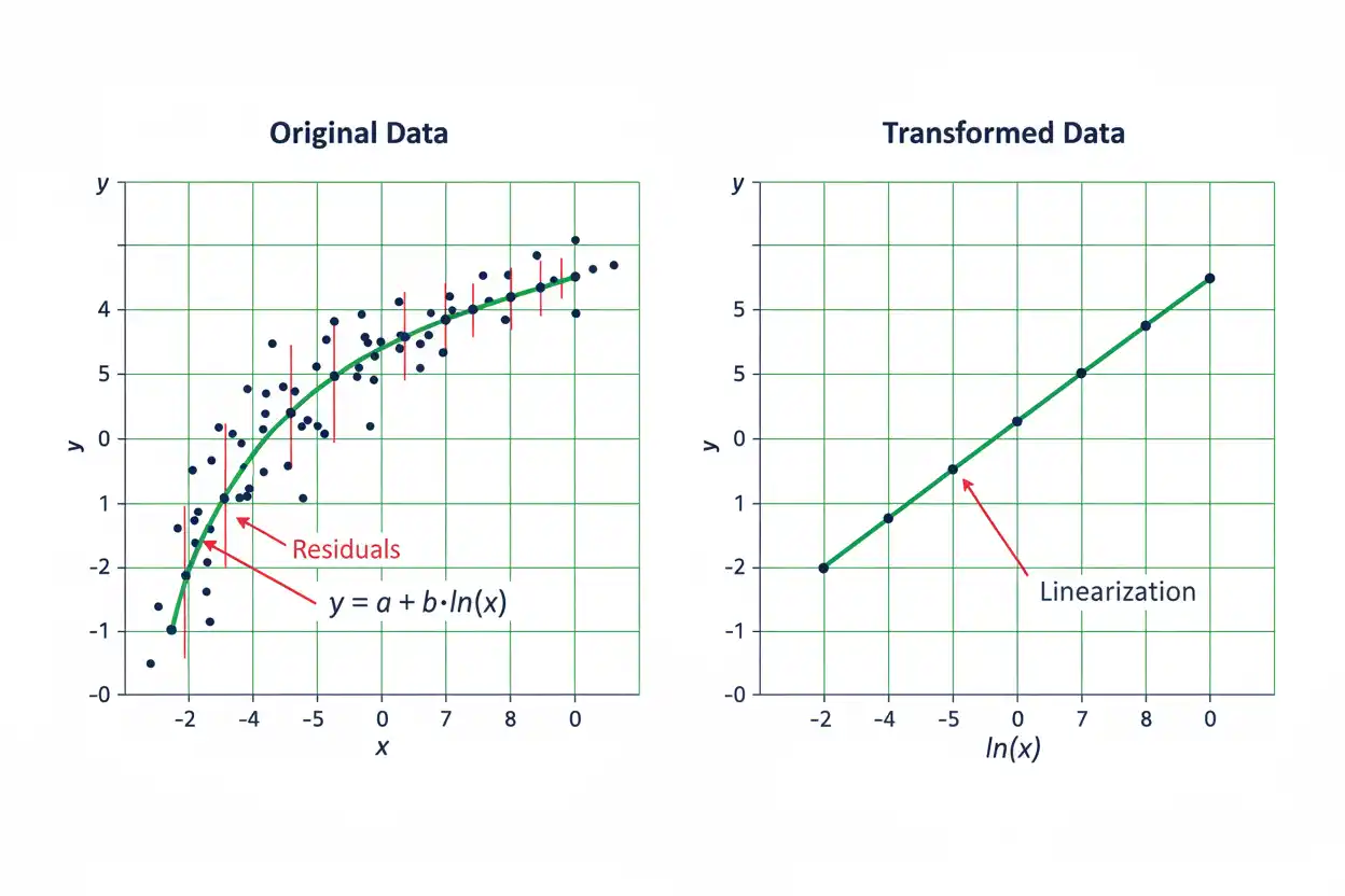
Logarithmic regression is a statistical modeling method used when a quantitative response changes rapidly at smaller predictor values and then changes progressively more slowly as the predictor grows. A common logarithmic regression model is ŷ = a + b ln(x), where x must be positive, a is the fitted response when x = 1, and b controls the direction and magnitude of change with respect to the logarithm of x. Unlike ordinary straight-line regression, equal absolute increases in x do not produce equal changes in the fitted response. Instead, equal multiplicative changes in x produce equal additive changes in ŷ. For example, doubling x always changes the fitted response by b ln(2), regardless of the starting value of x. A positive b produces an increasing curve that gradually flattens, while a negative b produces a decreasing logarithmic curve. The model can be estimated by transforming the predictor to ln(x) and then applying ordinary least squares to y versus ln(x). Its usefulness depends on whether the transformed relationship is reasonably linear, whether the residual assumptions are suitable, and whether predictions remain within a range where logarithmic behavior is substantively plausible.
Logarithmic regression belongs to the modeling methods within core statistics and the broader Statistics & Probability framework. It uses the same least-squares machinery as linear regression, but applies that machinery to a logarithmically transformed predictor rather than to x directly.
What Is Logarithmic Regression?
Logarithmic regression models a response y as a linear function of the logarithm of a positive predictor x.
The standard form is:
ŷ = a + b ln(x)
where:
- ŷ = predicted response
- x = predictor, with x > 0
- a = intercept on the ln(x) scale
- b = logarithmic regression coefficient
- ln(x) = natural logarithm of x
The model can also be written:
Y = β₀ + β₁ ln(X) + ε
for a population regression model, where ε represents random error.
The key feature is that the response changes quickly when x is small and progressively more slowly as x increases.
If:
b > 0
the curve rises and gradually flattens.
If:
b < 0
the curve falls and gradually flattens.
If:
b = 0
the fitted response is constant:
ŷ = a
Logarithmic Regression Formula
The fitted equation is:
ŷ = a + b ln(x)
To estimate a and b, define a transformed predictor:
z = ln(x)
The model becomes:
ŷ = a + bz
This is an ordinary simple linear regression in z.
The least-squares slope is:
b = Σ(zᵢ − z̄)(yᵢ − ȳ) / Σ(zᵢ − z̄)²
Because:
zᵢ = ln(xᵢ)
the same formula can be written directly as:
b = Σ[ln(xᵢ) − ln(x)̄](yᵢ − ȳ) / Σ[ln(xᵢ) − ln(x)̄]²
The intercept is:
a = ȳ − b ln(x)̄
where:
- ȳ = sample mean of the response values
- ln(x)̄ = mean of the transformed predictor values
Once a and b are estimated, predictions are calculated by substituting positive x values into:
ŷ = a + b ln(x)
Why x Must Be Positive
The real-valued natural logarithm is defined only for:
x > 0
Therefore, ordinary logarithmic regression using ln(x) cannot directly include:
x = 0
or:
x < 0
because:
ln(0)
is undefined and:
ln(x)
has no real value for negative x.
This is not merely a computational inconvenience. It is a property of the model itself.
Adding an arbitrary constant to x solely to make all values positive changes the relationship being modeled:
ln(x)
becomes:
ln(x + c)
That is a different model with different parameters and interpretation.
Any such shift must therefore be substantively justified rather than treated as an automatic fix.
What Does the Intercept Mean?
In:
ŷ = a + b ln(x)
set:
x = 1
Because:
ln(1) = 0
we obtain:
ŷ = a
Therefore, the intercept a is the predicted response when:
x = 1
This differs from ordinary linear regression, where the intercept represents the fitted response at x = 0.
That distinction is important because x = 0 is not even inside the domain of an ordinary logarithmic regression.
For logarithmic regression:
a = predicted y at x = 1
provided x = 1 is meaningful in the application.
What Does the Coefficient b Mean?
The coefficient b describes how much the predicted response changes when ln(x) increases by one unit.
A one-unit increase in:
ln(x)
corresponds to multiplying x by:
e ≈ 2.71828
Therefore, multiplying x by e changes the fitted response by:
b
units.
If:
b = 4
then increasing x by a factor of e raises the predicted response by 4 units.
If:
b = −4
the same multiplicative increase in x lowers the predicted response by 4 units.
This interpretation is mathematically exact for the fitted logarithmic model.
Interpreting a Doubling of x
A particularly useful interpretation concerns doubling.
Suppose x changes from:
x
to:
2x
The original prediction is:
ŷ₁ = a + b ln(x)
The new prediction is:
ŷ₂ = a + b ln(2x)
Using:
ln(2x) = ln(2) + ln(x)
we obtain:
ŷ₂ − ŷ₁ = b ln(2)
Therefore:
Change from doubling x = b ln(2)
Since:
ln(2) ≈ 0.6931
a doubling changes the fitted response by approximately:
0.6931b
For example, if:
b = 5
then doubling x changes ŷ by:
5 × 0.6931 ≈ 3.466
So every doubling of x is associated with approximately a 3.47-unit change in the fitted response.
Interpreting a Percentage Increase in x
Suppose x increases by r percent.
The new predictor value is:
xnew = x(1 + r)
where r is written as a decimal.
The predicted change is:
Δŷ = b ln(1 + r)
For a 10% increase:
r = 0.10
so:
Δŷ = b ln(1.10)
Since:
ln(1.10) ≈ 0.09531
we obtain:
Δŷ ≈ 0.09531b
If:
b = 8
then a 10% increase in x changes the fitted response by approximately:
8 × 0.09531
≈ 0.7625
units.
This percentage interpretation is often more informative than describing a one-unit change in x because logarithmic regression is fundamentally based on proportional changes in the predictor.
Logarithmic Regression Example
Consider the following data:
| x | y |
|---|---|
| 1 | 2.2 |
| 2 | 4.0 |
| 4 | 6.3 |
| 8 | 7.9 |
| 16 | 10.1 |
The response rises rapidly at smaller x values and then increases by progressively smaller amounts for equal absolute changes in x.
We will fit:
ŷ = a + b ln(x)
Step 1: Transform x
Calculate the natural logarithm of each predictor value.
| x | y | ln(x) |
|---|---|---|
| 1 | 2.2 | 0.0000 |
| 2 | 4.0 | 0.6931 |
| 4 | 6.3 | 1.3863 |
| 8 | 7.9 | 2.0794 |
| 16 | 10.1 | 2.7726 |
Let:
z = ln(x)
The model is now:
ŷ = a + bz
Step 2: Calculate the Mean Values
The mean response is:
ȳ = (2.2 + 4.0 + 6.3 + 7.9 + 10.1)/5
ȳ = 6.1
The mean transformed predictor is:
z̄ = (0 + 0.6931 + 1.3863 + 2.0794 + 2.7726)/5
z̄ ≈ 1.3863
Step 3: Calculate the Slope
Use:
b = Σ(zᵢ − z̄)(yᵢ − ȳ) / Σ(zᵢ − z̄)²
For these observations:
b ≈ 2.8421
Step 4: Calculate the Intercept
a = ȳ − bz̄
Substitute:
a ≈ 6.1 − (2.8421)(1.3863)
a ≈ 2.16
Therefore, the fitted logarithmic regression equation is:
ŷ ≈ 2.16 + 2.8421 ln(x)
Interpreting the Example Equation
The intercept is:
a ≈ 2.16
so when:
x = 1
the model predicts:
ŷ ≈ 2.16
The logarithmic coefficient is:
b ≈ 2.8421
This means multiplying x by e increases the fitted response by approximately:
2.8421 units
A doubling of x changes the predicted response by:
2.8421 ln(2)
≈ 1.97
Therefore, each doubling of x is associated with approximately:
1.97 units
of additional fitted response.
That pattern can be seen directly in the example because x doubles at every step.
Predicted Values
Using:
ŷ = 2.16 + 2.8421 ln(x)
the predicted values are approximately:
| x | Observed y | Predicted ŷ |
|---|---|---|
| 1 | 2.2 | 2.16 |
| 2 | 4.0 | 4.13 |
| 4 | 6.3 | 6.10 |
| 8 | 7.9 | 8.07 |
| 16 | 10.1 | 10.04 |
The predicted values follow the observed pattern closely in this small illustrative data set.
The fact that the x values double each time makes the fitted y increments nearly constant because:
ln(2x) − ln(x) = ln(2)
at every step.
Calculating a Prediction
Suppose we want the predicted response when:
x = 10
Use:
ŷ = 2.16 + 2.8421 ln(10)
Since:
ln(10) ≈ 2.3026
we obtain:
ŷ ≈ 2.16 + 2.8421(2.3026)
ŷ ≈ 8.70
Therefore, the fitted logarithmic regression predicts approximately:
8.70
when x = 10.
Because 10 lies inside the observed range from 1 to 16, this is interpolation rather than extrapolation.
Residuals in Logarithmic Regression
A residual is:
eᵢ = yᵢ − ŷᵢ
For the example:
| x | y | ŷ | Residual |
|---|---|---|---|
| 1 | 2.2 | 2.16 | 0.04 |
| 2 | 4.0 | 4.13 | −0.13 |
| 4 | 6.3 | 6.10 | 0.20 |
| 8 | 7.9 | 8.07 | −0.17 |
| 16 | 10.1 | 10.04 | 0.06 |
The residuals are small in this example and alternate around zero without an obvious systematic pattern.
A real analysis should examine residuals more carefully for:
- curvature,
- changing spread,
- influential observations,
- clusters,
- dependence,
- omitted structure.
A visually good fitted curve alone does not establish that the statistical model is appropriate.
Sum of Squared Residuals
Ordinary least squares minimizes:
SSE = Σ(yᵢ − ŷᵢ)²
For the example:
SSE ≈ 0.091
This represents the remaining squared variation in the response after fitting the logarithmic relationship.
Because y itself was not transformed, the residuals and SSE are measured on the original y scale.
This point distinguishes logarithmic regression of the form:
y = a + b ln(x)
from log-linear exponential regression, where ln(y) may instead be the transformed response.
R² for Logarithmic Regression
The coefficient of determination can be calculated as:
R² = 1 − SSE/SST
where:
SST = Σ(yᵢ − ȳ)²
For the example:
SSE ≈ 0.091
and:
SST = 38.9
Therefore:
R² = 1 − 0.091/38.9
R² ≈ 0.9977
Thus approximately:
99.77%
of the observed sample variation in y around its mean is accounted for by the fitted relationship with ln(x).
This extremely high R² is intentionally produced by the small illustrative example and should not be treated as typical of real data.
What R² Means Here
Because logarithmic regression is fitted as:
y = a + b ln(x)
ordinary least squares is minimizing errors in the original response y.
Therefore, the standard R² for this model describes variation in:
y
not variation in ln(y).
This is an important distinction from some forms of exponential regression, where the response itself may be logarithmically transformed before fitting.
R² values calculated on different response scales should not be compared casually.
Logarithmic Regression vs Linear Regression
A standard linear regression has:
ŷ = a + bx
A logarithmic regression has:
ŷ = a + b ln(x)
In linear regression, the marginal effect of x is constant:
Change in ŷ per unit x = b
In logarithmic regression, the marginal effect decreases as x increases.
The derivative is:
dŷ/dx = b/x
Therefore, if:
b > 0
the response continues to rise, but each additional unit of x has a smaller fitted effect.
For example, increasing x from 1 to 2 generally changes ŷ much more than increasing x from 101 to 102.
That declining marginal effect is one of the defining features of logarithmic regression.
Constant Differences vs Constant Ratios
Linear and logarithmic regression behave differently when x changes.
With linear regression:
Equal differences in x → equal changes in ŷ
With logarithmic regression:
Equal ratios in x → equal changes in ŷ
Suppose x doubles:
1 → 2
5 → 10
50 → 100
In a logarithmic model, every doubling changes the prediction by:
b ln(2)
regardless of the starting x value.
This multiplicative interpretation makes logarithmic regression especially natural when proportional rather than absolute changes in x matter.
Logarithmic Regression vs Exponential Regression
The two models are often confused because logarithms can appear in both fitting procedures.
Logarithmic regression has the form:
y = a + b ln(x)
Here, the predictor is logarithmically transformed.
Exponential regression commonly has:
y = abˣ
and may be linearized as:
ln(y) = ln(a) + x ln(b)
Here, the response is logarithmically transformed in the linearized fitting method.
The shapes also differ.
A positive logarithmic regression tends to rise rapidly and flatten.
A positive exponential regression tends to rise increasingly rapidly.
They represent almost opposite forms of curvature.
Shape of a Positive Logarithmic Regression
Suppose:
b > 0
Then:
dŷ/dx = b/x > 0
so the fitted curve is increasing.
The second derivative is:
d²ŷ/dx² = −b/x²
which is negative.
Therefore, the curve is concave downward.
It rises rapidly at smaller values of x and then progressively flattens.
As:
x → ∞
the slope:
b/x
approaches:
0
although ln(x) itself continues to increase without bound.
Thus, the fitted response continues increasing, but increasingly slowly.
Shape of a Negative Logarithmic Regression
If:
b < 0
then:
dŷ/dx = b/x < 0
for x > 0.
The fitted response decreases as x increases.
However, the magnitude of the slope:
|b|/x
becomes smaller as x grows.
Therefore, the curve falls quickly at small x values and then flattens.
A negative logarithmic regression can be useful when a response declines sharply initially but later reductions become progressively smaller.
Behavior Near x = 0
The natural logarithm has:
ln(x) → −∞
as:
x → 0⁺
Therefore, the logarithmic regression curve can become extreme near zero.
If:
b > 0
then:
a + b ln(x) → −∞
as x approaches zero from the positive side.
If:
b < 0
the predicted response tends toward positive infinity.
In many real applications this behavior is unrealistic.
Therefore, logarithmic regression should not be extrapolated toward x = 0 merely because the equation mathematically permits positive values arbitrarily close to zero.
Why Logarithmic Regression Flattens
Consider two one-unit changes.
First:
x = 1 → x = 2
The transformed change is:
ln(2) − ln(1)
≈ 0.6931
Now consider:
x = 100 → x = 101
The transformed change is:
ln(101) − ln(100)
≈ 0.00995
The second change is much smaller on the logarithmic scale.
Therefore, the same one-unit increase in x produces a much smaller change in the fitted response when x is already large.
This is the mathematical basis of diminishing marginal effects in logarithmic regression.
Natural Log vs Base-10 Log
A logarithmic model does not have to use the natural logarithm.
One could instead fit:
ŷ = A + B log₁₀(x)
Because:
ln(x) = ln(10) log₁₀(x)
the two forms can describe the same fitted curve after coefficients are converted appropriately.
If:
y = a + b ln(x)
then:
y = a + [b ln(10)] log₁₀(x)
Therefore, changing the log base changes the numerical slope coefficient but not the underlying family of fitted curves when the transformation is handled consistently.
The natural logarithm is standard in much of statistics because of its mathematical convenience.
Solving the Model for x
Sometimes the fitted equation must be inverted.
Start with:
y = a + b ln(x)
Assuming:
b ≠ 0
subtract a:
y − a = b ln(x)
Divide by b:
ln(x) = (y − a)/b
Exponentiate:
x = exp[(y − a)/b]
This allows the predictor value corresponding to a specified fitted response to be calculated.
Such inverse predictions should be interpreted cautiously because ordinary least squares was fitted to predict y from x, not necessarily x from y.
Assumptions of Logarithmic Regression
Once:
z = ln(x)
has been defined, logarithmic regression becomes an ordinary linear model in z.
The usual regression considerations therefore apply to:
Y = β₀ + β₁Z + ε
where:
Z = ln(X)
Appropriate Functional Form
The conditional mean should be reasonably represented by:
E(Y|X=x) = β₀ + β₁ ln(x)
A curved scatter plot alone does not prove that a logarithmic model is appropriate.
Residual behavior and subject-matter reasoning should support the transformation.
Independence
Under conventional regression inference, observations or errors should follow the assumed independence structure.
Repeated measurements, time-dependent data, or clusters may require methods that model dependence explicitly.
Constant Error Variance
Classical ordinary least squares commonly assumes:
Var(ε|X=x) = σ²
If residual variability grows or shrinks systematically with x, conventional standard errors may be inappropriate.
Zero Conditional Mean
A core assumption is:
E(ε|X) = 0
Systematic omitted factors associated with x can bias the fitted coefficient.
Error Distribution for Small-Sample Classical Inference
Exact small-sample t and F inference is commonly developed under normally distributed model errors.
The raw x values themselves do not need to be normally distributed.
Logarithmic Regression Does Not Require Normal x
The predictor x can be strongly skewed.
In fact, logarithmic regression is often considered precisely because the predictor spans a wide positive range.
The transformed quantity:
ln(x)
enters the linear regression equation.
There is no requirement that x itself follow a normal distribution.
Nor is there a general requirement that ln(x) itself be normally distributed merely to calculate the least-squares coefficients.
Distributional assumptions matter primarily for particular inferential procedures and error models.
Residual Diagnostics
After fitting logarithmic regression, examine residuals against:
- fitted values,
- x,
- ln(x),
- observation order when relevant.
A residual plot should not show strong systematic structure if the logarithmic mean function is appropriate.
For example, if residuals curve downward and then upward, the logarithmic model may still be missing important nonlinear structure.
A funnel shape can suggest nonconstant variance.
Clusters can indicate subgroups or omitted predictors.
Residual analysis is more informative than relying solely on a high R².
Outliers and Logarithmic Regression
Unusual observations can materially influence logarithmic regression.
Because:
ln(x)
compresses large positive x values, the leverage pattern differs from regression on raw x.
At the same time, values very close to zero can be far away on the ln(x) scale.
For example:
ln(0.01) ≈ −4.605
while:
ln(1) = 0
An x value near zero can therefore have substantial leverage on the transformed scale.
Unusual y values can also create large residuals.
An interquartile range rule can help identify unusual univariate observations, but it cannot determine by itself whether a point is influential in the fitted regression.
Mean Absolute Deviation and Residuals
Ordinary least squares fits logarithmic regression by minimizing squared residuals.
However, descriptive summaries of residual magnitudes can also help communicate prediction error.
The mean absolute deviation framework uses absolute distances rather than squared distances.
For regression residuals, an average absolute error can be calculated as:
MAE = Σ|eᵢ|/n
For the worked example:
|e| ≈ 0.04, 0.13, 0.20, 0.17, 0.06
so:
MAE ≈ (0.04 + 0.13 + 0.20 + 0.17 + 0.06)/5
MAE ≈ 0.12
This does not replace the least-squares objective, but it provides an alternative descriptive view of typical absolute prediction error.
Statistical Inference for b
The population logarithmic regression model is:
Y = β₀ + β₁ ln(X) + ε
A common hypothesis test asks:
H₀: β₁ = 0
against:
H₁: β₁ ≠ 0
If:
β₁ = 0
the conditional mean does not change with ln(x) under the specified model.
The test statistic typically has the form:
t = b/SE(b)
when the null value is zero.
For simple logarithmic regression under the conventional framework:
df = n − 2
The resulting p-value should be interpreted in the usual frequentist way: it describes how extreme the observed statistic would be under H₀ and the assumed reference model, not the probability that H₀ itself is true.
Confidence Interval for the Logarithmic Coefficient
A confidence interval for β₁ can be written:
b ± t*SE(b)
under the standard t-based procedure.
The interval describes uncertainty in the population coefficient governing change with respect to ln(x).
Suppose a 95% interval for b is:
(1.8, 3.9)
Because the interval excludes zero, the corresponding two-sided test would ordinarily reject:
H₀: β₁ = 0
at α = 0.05 under compatible procedures.
The interval is more informative than a binary significance decision because it also shows the plausible magnitude of the coefficient under the method.
Statistical Significance vs Practical Significance
A logarithmic regression coefficient can be statistically significant while implying a very small practical effect.
Suppose:
b = 0.05
in an enormous sample.
A doubling of x changes the fitted response by:
0.05 ln(2)
≈ 0.0347
units.
That effect may be statistically distinguishable from zero while remaining practically negligible.
Conversely, a larger coefficient in a small sample can have substantial uncertainty and fail to reach a conventional significance threshold.
Effect magnitude, uncertainty, and practical consequences should therefore be considered separately from statistical significance.
Logarithmic Regression and Causation
A fitted logarithmic relationship does not prove that x causes y.
Suppose:
y = a + b ln(x)
fits the observations extremely well.
Possible explanations still include:
- x influencing y,
- y influencing x indirectly,
- a third variable influencing both,
- selection effects,
- common trends,
- measurement structure,
- chance or model misspecification.
Regression describes conditional association unless a research design and assumptions justify a stronger causal interpretation.
A high R² does not change this limitation.
Interpolation
Interpolation uses the fitted equation for predictor values inside the observed x range.
In the worked example:
1 ≤ x ≤ 16
Predicting at:
x = 10
is interpolation.
Because the prediction is supported by nearby observed x values, interpolation is generally safer than extrapolation.
However, even an interpolated prediction can be unreliable if the model form, error structure, or data quality is poor.
Being inside the observed range does not guarantee correctness.
Extrapolation
Predicting beyond the observed x range is extrapolation.
For example, using a model fitted over:
1 ≤ x ≤ 16
to predict:
x = 1,000
requires assuming the logarithmic relationship continues far beyond the data.
The equation will produce a numerical prediction:
ŷ = a + b ln(1,000)
but the real process may flatten completely, reverse, encounter physical limits, or follow another relationship.
Extrapolation toward zero is particularly dangerous because ln(x) diverges as x approaches zero from above.
When Logarithmic Regression Is Appropriate
Logarithmic regression can be a useful candidate when:
- x is positive,
- y changes quickly at lower x values,
- the marginal effect of x declines as x increases,
- equal proportional changes in x produce approximately equal changes in y,
- plotting y against ln(x) gives an approximately linear pattern,
- residual diagnostics support the model,
- the underlying process makes diminishing effects plausible.
Examples can arise in learning curves, diminishing returns, response saturation over limited ranges, and relationships spanning several orders of magnitude.
However, the functional form should be supported rather than chosen only because it produces a high R².
When Logarithmic Regression Is Not Appropriate
The model may be unsuitable when:
- x includes zero or negative values that have meaningful roles,
- the relationship is approximately linear in raw x,
- the response accelerates rather than flattens,
- the data clearly approach a finite asymptote,
- residuals show systematic curvature,
- observations are dependent in an unmodeled way,
- a few influential observations create the apparent shape,
- extrapolation would imply impossible values.
A flattening relationship is not automatically logarithmic. Other models can also display diminishing slopes.
Logarithmic Regression vs a Geometric Distribution
A geometric distribution is a discrete probability distribution for waiting until a first success.
Logarithmic regression is a regression model for the mean relationship between a quantitative response and a positive predictor.
These methods answer completely different questions.
The geometric distribution assigns probabilities to integer waiting times.
Logarithmic regression calculates fitted response values such as:
ŷ = a + b ln(x)
The appearance of nonlinear mathematical functions in both statistical topics does not make one a substitute for the other.
Changing the Units of x
Logarithmic regression has an interesting unit-transformation property.
Suppose x is multiplied by a positive constant c:
x* = cx
Then:
ln(x*) = ln(cx)
= ln(c) + ln(x)
Substitute into the model:
y = a + b ln(x*)
= a + b ln(c) + b ln(x)
The coefficient on ln(x) remains:
b
while the intercept shifts.
Therefore, changing x between proportional units can leave the logarithmic slope unchanged while altering the intercept.
For example, changing a positive predictor from meters to centimeters changes its scale by a factor of 100 and therefore shifts the intercept by a term involving:
b ln(100)
The fitted predictions remain consistent when the transformation is handled correctly.
Scaling y
If the response y is multiplied by a constant, both the intercept and slope change correspondingly.
For:
y* = cy
the fitted relationship becomes:
ŷ* = ca + cb ln(x)
Therefore, the coefficient b retains the measurement units of y.
It is not standardized.
A coefficient of:
b = 5 kilograms
and one of:
b = 5 grams
do not represent the same magnitude.
Units should be considered when interpreting logarithmic regression coefficients.
Does Logarithmic Regression Have an Asymptote?
The function:
y = a + b ln(x)
has a vertical boundary at:
x = 0
because ln(x) is undefined there.
As:
x → 0⁺
ln(x) tends toward negative infinity.
However, a positive logarithmic model does not have a finite horizontal asymptote as x increases.
Although its slope approaches zero:
b/x → 0
the logarithm continues increasing without bound.
Therefore, a logarithmic model keeps increasing for b > 0, just very slowly.
This distinguishes it from models that truly approach a finite upper limit.
Logarithmic Regression and Diminishing Returns
A positive logarithmic regression naturally represents diminishing marginal effects because:
dŷ/dx = b/x
When x doubles, the slope at the new x is half the slope at the old x.
For example, with:
b = 10
the instantaneous slope at:
x = 2
is:
10/2 = 5
while at:
x = 20
it is:
10/20 = 0.5
Thus, additional units of x have progressively smaller fitted effects as x becomes larger.
This pattern is mathematically consistent with diminishing returns over a range where a logarithmic approximation is substantively reasonable.
Common Logarithmic Regression Mistakes
A common mistake is confusing logarithmic regression with exponential regression. Logarithmic regression transforms x, while a common exponential fitting approach transforms y.
Another mistake is including:
x = 0
inside ln(x), even though the logarithm is undefined there.
A third error is interpreting b as the change in y for a one-unit increase in raw x. The raw-x marginal effect is:
b/x
not a constant b.
It is also incorrect to say that a positive logarithmic curve reaches a finite maximum merely because it flattens. The slope approaches zero, but ln(x) continues increasing.
Another mistake is comparing R² values from models fitted on different response scales without recognizing what variation each statistic measures.
Analysts can also overinterpret a high R² while ignoring residual patterns, influential observations, dependence, or implausible extrapolation.
Finally, a statistically significant logarithmic coefficient should not be treated as evidence of causation or practical importance without additional analysis.
How to Calculate Logarithmic Regression Step by Step
A standard calculation follows this process.
Step 1: Verify the Predictor Domain
Confirm:
xᵢ > 0
for every observation.
Step 2: Transform the Predictor
Calculate:
zᵢ = ln(xᵢ)
Step 3: Calculate Means
Find:
z̄ = Σzᵢ/n
and:
ȳ = Σyᵢ/n
Step 4: Calculate the Slope
b = Σ(zᵢ − z̄)(yᵢ − ȳ) / Σ(zᵢ − z̄)²
Step 5: Calculate the Intercept
a = ȳ − bz̄
Step 6: Write the Model
ŷ = a + b ln(x)
Step 7: Calculate Predictions
Substitute positive x values into the fitted equation.
Step 8: Calculate Residuals
eᵢ = yᵢ − ŷᵢ
Step 9: Assess Fit
Examine:
- residual structure,
- R²,
- influential points,
- uncertainty,
- domain restrictions,
- substantive plausibility.
Step 10: Interpret Multiplicative Changes Correctly
For a multiplier k:
Δŷ = b ln(k)
This is often more informative than trying to interpret a constant one-unit raw-x effect.
How to Report Logarithmic Regression
A useful report should state the fitted equation and interpret b in meaningful terms.
For the worked example:
ŷ ≈ 2.16 + 2.8421 ln(x)
A practical interpretation is:
Doubling x is associated with an estimated increase of approximately 1.97 units in the fitted response.
The model has:
R² ≈ 0.9977
in the small illustrative sample.
A real inferential report may additionally include:
- sample size,
- standard error of b,
- confidence interval,
- test statistic,
- degrees of freedom,
- p-value,
- residual diagnostics.
The language should describe association unless the study design supports causal conclusions.
Frequently Asked Questions About Logarithmic Regression
What is logarithmic regression?
Logarithmic regression models a quantitative response as a linear function of the logarithm of a positive predictor.
What is the logarithmic regression formula?
A common form is:
ŷ = a + b ln(x)
with:
x > 0
What does a represent?
Because:
ln(1) = 0
a is the predicted response when:
x = 1
What does b represent?
b is the predicted change in y when ln(x) increases by one unit, which is equivalent to multiplying x by e.
What happens when x doubles?
The fitted response changes by:
b ln(2)
or approximately:
0.6931b
How do you interpret a 10% increase in x?
The fitted response changes by:
b ln(1.10)
which is approximately:
0.09531b
Why must x be positive?
The real natural logarithm ln(x) is defined only for:
x > 0
so zero and negative predictor values cannot be used directly in the ordinary logarithmic model.
Can logarithmic regression use x = 0?
No. ln(0) is undefined.
Can logarithmic regression use negative x values?
Not with the standard real-valued ln(x) transformation.
How is logarithmic regression calculated?
Transform the predictor:
z = ln(x)
then fit the ordinary linear regression:
y = a + bz
using least squares.
What is the slope formula?
b = Σ(zᵢ − z̄)(yᵢ − ȳ) / Σ(zᵢ − z̄)²
where:
zᵢ = ln(xᵢ)
What is the difference between logarithmic and linear regression?
Linear regression assumes constant additive change for equal raw-x changes. Logarithmic regression assumes equal multiplicative changes in x correspond to equal additive changes in the fitted response.
What is the difference between logarithmic and exponential regression?
Logarithmic regression commonly uses:
y = a + b ln(x)
while exponential regression commonly uses:
y = abˣ
A positive logarithmic curve flattens as x increases, while a positive exponential curve becomes progressively steeper.
Does logarithmic regression always flatten?
For b ≠ 0, the absolute slope is:
|b|/x
which approaches zero as x grows. The curve therefore becomes progressively flatter.
Does a positive logarithmic regression have a maximum value?
No. It continues increasing without bound as x increases, although its slope approaches zero.
What is the derivative of a logarithmic regression?
For:
y = a + b ln(x)
the derivative is:
dy/dx = b/x
Can logarithmic regression be used for prediction?
Yes, provided x is positive and the model is appropriate. Predictions far outside the observed predictor range should be treated cautiously.
What does R² mean in logarithmic regression?
When y is regressed directly on ln(x), R² describes the proportion of sample variation in y around its mean accounted for by the fitted model.
Does a high R² prove logarithmic regression is correct?
No. Residual behavior, competing models, influential observations, assumptions, and substantive plausibility must also be considered.
Does logarithmic regression prove causation?
No. It describes an association pattern unless a research design and additional assumptions justify causal interpretation.
Can outliers affect logarithmic regression?
Yes. Unusual y values and extreme values on the ln(x) scale can substantially influence fitted coefficients and predictions.
Is logarithmic regression a probability distribution?
No. It is a regression model. Probability distributions such as the geometric distribution answer different statistical questions.
When is logarithmic regression useful?
It can be useful when x is positive, effects are strongest at smaller x values, marginal effects decline as x increases, and proportional changes in x are more meaningful than equal absolute changes.




