

Exponential Regression: Definition, Formula & Example

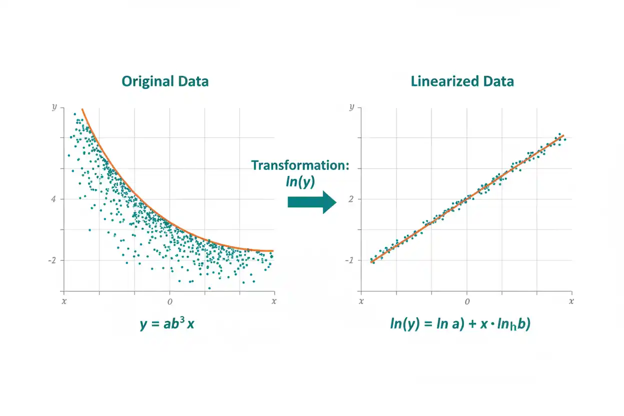
Exponential regression is a statistical modeling method used when a quantitative response changes approximately by a constant multiplicative factor rather than by a constant additive amount. Instead of fitting a straight-line relationship such as y = a + bx, exponential regression fits a curved model in which equal increases in x correspond to proportional increases or decreases in y. A common form is y = abˣ, where a determines the value when x = 0 and b controls the rate and direction of exponential change. Values of b greater than 1 describe exponential growth, while values between 0 and 1 describe exponential decay. The model can often be estimated by transforming positive response values with the natural logarithm and fitting a linear relationship between x and ln(y), although that approach minimizes error on the logarithmic scale rather than the original response scale. Exponential regression is useful when the data genuinely support multiplicative change, but a visually curved pattern alone is not enough to justify it. Residual behavior, domain knowledge, extrapolation risk, error structure, outliers, and comparison with plausible competing models all matter when deciding whether exponential regression is appropriate.
Within core statistics, exponential regression extends regression modeling beyond constant additive change. The broader Statistics & Probability framework includes descriptive measures, probability distributions, inference, association, and other tools that help determine whether an exponential model is statistically and substantively reasonable.
What Is Exponential Regression?
Exponential regression models a response variable y as an exponential function of an explanatory variable x.
A common model is:
y = abˣ
where:
- y = predicted response
- x = explanatory variable
- a = initial value or scale parameter
- b = multiplicative change factor per one-unit increase in x
For a valid basic exponential model:
a > 0
and:
b > 0
If:
b > 1
the model represents exponential growth.
If:
0 < b < 1
the model represents exponential decay.
If:
b = 1
then:
y = a
for every x, so the model is constant rather than meaningfully exponential.
The defining feature is that the ratio between predictions at successive one-unit x values is constant:
y(x + 1)/y(x) = b
That differs fundamentally from linear regression, where equal increases in x correspond to a constant additive change in y.
Exponential Regression Formula
The basic form is:
ŷ = abˣ
The hat over y indicates a fitted or predicted value.
An equivalent form uses the natural exponential function:
ŷ = aeᵏˣ
where:
k = ln(b)
and therefore:
b = eᵏ
These parameterizations describe the same family of curves.
For example, if:
b = 1.08
then:
k = ln(1.08)
k ≈ 0.07696
so:
y = a(1.08)ˣ
can also be written approximately as:
y = ae⁰·⁰⁷⁶⁹⁶ˣ
The first form is often easier to interpret as a per-unit multiplicative factor, while the second is useful when working with continuous exponential growth rates.
Meaning of the Parameter a
In:
y = abˣ
set:
x = 0
Then:
y = ab⁰
Since:
b⁰ = 1
we obtain:
y = a
Therefore, a is the model’s predicted response when:
x = 0
This interpretation is meaningful only when x = 0 makes sense in the context of the data.
For example, if x represents years since the start of an experiment, a can represent the fitted starting value.
If x represents calendar year directly, x = 0 may lie far outside the observed data and a may have little practical interpretation even though it remains mathematically necessary.
Meaning of the Parameter b
The parameter b is the multiplicative factor associated with a one-unit increase in x.
From:
y(x) = abˣ
and:
y(x + 1) = abˣ⁺¹
we have:
y(x + 1)/y(x) = b
Therefore:
y(x + 1) = b × y(x)
If:
b = 1.20
each one-unit increase in x multiplies the fitted response by:
1.20
which corresponds to a 20% increase.
If:
b = 0.80
each one-unit increase multiplies the response by:
0.80
which corresponds to a 20% decrease.
This multiplicative interpretation is central to exponential regression.
Growth Rate From b
When:
b > 1
the proportional growth rate per unit of x is:
r = b − 1
The percentage growth rate is:
Growth rate (%) = (b − 1) × 100%
For example, if:
b = 1.15
then:
r = 1.15 − 1 = 0.15
so the fitted response grows by:
15%
for each one-unit increase in x.
This interpretation assumes that x advances in equal units.
If x is measured in months, b describes a per-month factor. If x is measured in years, it describes a per-year factor.
Decay Rate From b
When:
0 < b < 1
the model decreases exponentially.
For example:
b = 0.92
means each one-unit increase in x multiplies the response by:
0.92
The proportional decline is:
1 − 0.92 = 0.08
or:
8%
per unit of x.
The fitted values never become negative under this model as long as a > 0 and b > 0.
They instead approach zero as x increases when 0 < b < 1.
Exponential Regression and the Natural Exponential Form
Another common model is:
y = aeᵏˣ
The parameter k is a continuous exponential rate.
If:
k > 0
the model grows.
If:
k < 0
the model decays.
The relationship between the two forms is:
b = eᵏ
and:
k = ln(b)
Therefore:
abˣ = aeˣˡⁿ⁽ᵇ⁾
Both forms produce exactly the same predicted values when their parameters are converted correctly.
How Exponential Regression Can Be Linearized
For positive y values, start with:
y = abˣ
Take the natural logarithm of both sides:
ln(y) = ln(abˣ)
Using logarithm rules:
ln(y) = ln(a) + x ln(b)
Define:
Y* = ln(y)
c = ln(a)
m = ln(b)
Then:
Y* = c + mx
This is a linear relationship between x and ln(y).
A straight-line regression can therefore be fitted to:
x
and:
ln(y)
The fitted intercept c and slope m can then be transformed back:
a = eᶜ
b = eᵐ
This is a common way to estimate an exponential regression model.
Why y Must Be Positive for Log Transformation
The logarithmic transformation requires:
y > 0
because the real-valued natural logarithm is undefined for:
y ≤ 0
Therefore, the log-linear fitting method cannot be applied directly when the response includes zeros or negative values.
Simply adding an arbitrary constant to every y value so that logarithms become possible changes the model itself and can distort interpretation.
If the data include zero or negative responses, another functional form or a directly fitted nonlinear model may be more appropriate.
Exponential Regression Example
Consider the following observations:
| x | y |
|---|---|
| 0 | 2.1 |
| 1 | 3.0 |
| 2 | 4.7 |
| 3 | 6.8 |
| 4 | 10.5 |
The response appears to increase at an accelerating rate, so an exponential regression model is a reasonable candidate.
We will fit:
y = abˣ
using the logarithmic transformation.
Step 1: Transform y
Calculate:
ln(y)
for each observation.
| x | y | ln(y) |
|---|---|---|
| 0 | 2.1 | 0.7419 |
| 1 | 3.0 | 1.0986 |
| 2 | 4.7 | 1.5476 |
| 3 | 6.8 | 1.9169 |
| 4 | 10.5 | 2.3514 |
We now fit the linear model:
ln(y) = c + mx
Step 2: Estimate the Linearized Slope
The ordinary least-squares slope is:
m = Σ(xᵢ − x̄)(ln(yᵢ) − ln(y)̄) / Σ(xᵢ − x̄)²
For these observations:
m ≈ 0.40372
Step 3: Estimate the Linearized Intercept
The intercept is:
c = ln(y)̄ − mx̄
which gives:
c ≈ 0.72384
Therefore, the fitted transformed model is:
ln(ŷ) ≈ 0.72384 + 0.40372x
Step 4: Convert Back to Exponential Parameters
Because:
a = eᶜ
we obtain:
a = e⁰·⁷²³⁸⁴
a ≈ 2.06235
And because:
b = eᵐ
we obtain:
b = e⁰·⁴⁰³⁷²
b ≈ 1.49738
Therefore, the fitted exponential regression equation is:
ŷ ≈ 2.06235(1.49738)ˣ
Rounded for interpretation:
ŷ ≈ 2.06(1.497)ˣ
Interpreting the Example
The fitted initial value is approximately:
a ≈ 2.06
so the model predicts:
ŷ ≈ 2.06
when:
x = 0
The multiplicative factor is:
b ≈ 1.49738
This means each one-unit increase in x multiplies the fitted response by approximately:
1.49738
The implied percentage increase is:
(1.49738 − 1) × 100%
≈ 49.74%
Thus, the model represents approximately 49.74% multiplicative growth per unit of x.
This does not mean the response increases by the same absolute amount each time. The absolute increases become larger because each new level is multiplied by the same factor.
Predicted Values From the Model
Using:
ŷ ≈ 2.06235(1.49738)ˣ
the fitted values are approximately:
| x | Observed y | Predicted ŷ |
|---|---|---|
| 0 | 2.1 | 2.062 |
| 1 | 3.0 | 3.088 |
| 2 | 4.7 | 4.624 |
| 3 | 6.8 | 6.924 |
| 4 | 10.5 | 10.368 |
The predictions closely match the observed data in this deliberately compact example.
However, model quality should not be judged simply by visual closeness over five observations. Residual structure, sample size, uncertainty, alternative functional forms, and the underlying process remain important.
Making a Prediction With Exponential Regression
Suppose we want the fitted response at:
x = 5
Use:
ŷ = 2.06235(1.49738)⁵
This gives approximately:
ŷ ≈ 15.52
Therefore, the exponential regression model predicts a response of about:
15.52
at x = 5.
If x = 5 lies just beyond an observed range of 0 through 4, this is technically extrapolation.
Even modest extrapolation should be interpreted cautiously because exponential models can grow or decay rapidly outside the fitted range.
Exponential Growth vs Linear Growth
Linear regression commonly has the form:
y = a + bx
The quantity b represents a constant additive change.
For example:
y = 10 + 3x
increases by exactly:
3 units
whenever x increases by 1.
Exponential regression instead has:
y = abˣ
where b represents a constant multiplicative change.
For example:
y = 10(1.20)ˣ
increases by:
20%
at each step.
The distinction is:
Linear model → constant difference
Exponential model → constant ratio
That is the most important conceptual difference between exponential and linear growth.
Exponential Regression vs Linear Regression
The choice between exponential regression and linear regression should depend on the relationship represented by the data and the underlying process.
A linear model is appropriate when:
Δy
is approximately constant for equal changes in x.
An exponential model is more appropriate when:
y₂/y₁
is approximately constant across equal x intervals.
For example, values:
10, 20, 30, 40
show constant additive change:
+10, +10, +10
which is linear.
Values:
10, 20, 40, 80
show constant multiplicative change:
×2, ×2, ×2
which is exponential.
Real data rarely follow either pattern perfectly, so regression is used to estimate the underlying trend rather than require exact equality.
Exponential Regression vs Logarithmic Regression
Exponential regression and logarithmic regression describe very different shapes.
An exponential model commonly has:
y = abˣ
A logarithmic model commonly has:
y = a + b ln(x)
Exponential growth can accelerate rapidly as x increases.
A logarithmic relationship changes quickly at first and then tends to flatten as x becomes larger.
These models should not be confused merely because logarithms appear in the calculation of exponential regression.
Taking:
ln(y)
to linearize an exponential model is a fitting transformation.
It does not turn the original relationship into logarithmic regression.
Exponential Regression and Correlation
After transforming an exponential model:
ln(y) = ln(a) + x ln(b)
the linear association between:
x
and:
ln(y)
can be examined using the correlation coefficient.
In the worked example, the sample correlation between x and ln(y) is approximately:
r ≈ 0.9994
This indicates an extremely strong positive linear association on the transformed scale.
However, a high transformed correlation does not automatically prove that exponential regression is the correct substantive model.
Different transformations can sometimes produce strong apparent linear relationships, especially with small samples.
Model choice still requires residual analysis, theoretical plausibility, and comparison with reasonable alternatives.
Exponential Regression and Covariance
The slope of the transformed regression can be expressed using covariance.
For the transformed response:
z = ln(y)
the fitted slope is:
m = Cov(x, z)/Var(x)
using compatible sample or population quantities.
Because:
m = ln(b)
we then obtain:
b = eᵐ
This shows how covariance contributes mathematically to exponential regression after logarithmic transformation.
The raw covariance between x and y alone does not determine the exponential model, because exponential regression concerns a nonlinear relationship on the original response scale.
R² in Exponential Regression
An R² value can be useful, but its interpretation depends on how the model was fitted.
If the model is estimated by applying ordinary least squares to:
ln(y)
then the usual regression R² describes variation explained on the logarithmic response scale.
For the worked example, the transformed-scale R² is approximately:
R²log ≈ 0.9988
If predicted values are transformed back and an R²-like measure is calculated from squared errors in the original y scale, the numerical result can differ.
For the same example, an original-scale calculation gives approximately:
R²original ≈ 0.9989
These happen to be very similar here because the model fits exceptionally closely.
They are not guaranteed to be equal in general.
An analyst should always state or understand which scale an R² refers to.
Why Log-Linear Fitting and Nonlinear Fitting Are Not Identical
Transforming:
y = abˣ
into:
ln(y) = ln(a) + x ln(b)
allows ordinary least squares to be applied conveniently.
However, fitting on the logarithmic scale minimizes:
Σ[ln(yᵢ) − ln(ŷᵢ)]²
It does not minimize:
Σ(yᵢ − ŷᵢ)²
on the original response scale.
Direct nonlinear least squares can instead estimate a and b by minimizing original-scale squared residuals.
The two approaches can therefore produce different parameter estimates.
Neither is universally superior. The appropriate method depends on the assumed error structure and the objective of the analysis.
Additive vs Multiplicative Errors
An important modeling decision concerns how random error behaves.
An additive-error model can be written conceptually as:
y = abˣ + ε
Here, the magnitude of the random error is treated on the original response scale.
A multiplicative-error model might instead be represented as:
y = abˣ × ε
Taking logarithms gives:
ln(y) = ln(a) + x ln(b) + ln(ε)
This structure is naturally compatible with regression on ln(y).
If variability increases proportionally with the fitted response, a multiplicative-error model may be plausible.
If errors have roughly constant absolute spread across y values, direct nonlinear fitting on the original scale may better match the data.
Back-Transformation Bias
When a regression model is fitted to ln(y), simply exponentiating the predicted log value produces an estimate associated with the geometric center of the conditional distribution rather than automatically recovering the arithmetic conditional mean.
If transformed residuals are approximately normal with nonzero variance, naive back-transformation can underestimate the mean response.
Under a simple lognormal error model with residual variance σ²ε:
E(Y|X=x) = exp[predicted ln(Y) + σ²ε/2]
rather than merely:
exp[predicted ln(Y)]
More general correction methods can also be used.
This issue matters when the purpose of exponential regression is to estimate expected values on the original scale rather than medians or typical multiplicative levels.
Residuals in Exponential Regression
A residual on the original scale is:
eᵢ = yᵢ − ŷᵢ
For the worked example, the approximate original-scale residuals are:
| x | Observed y | Predicted ŷ | Residual |
|---|---|---|---|
| 0 | 2.1 | 2.062 | 0.038 |
| 1 | 3.0 | 3.088 | −0.088 |
| 2 | 4.7 | 4.624 | 0.076 |
| 3 | 6.8 | 6.924 | −0.124 |
| 4 | 10.5 | 10.368 | 0.132 |
If the model was fitted on the logarithmic scale, transformed residuals are also important:
elog,i = ln(yᵢ) − ln(ŷᵢ)
Residual analysis should look for systematic curvature, changing variance, clusters, influential points, or other patterns suggesting that the assumed exponential form is inadequate.
What a Good Residual Pattern Looks Like
A useful regression model generally leaves residuals without a clear systematic pattern.
If residuals versus x form a curved structure, the exponential function may not describe the relationship adequately.
If residual spread grows substantially with fitted values on the original scale, multiplicative error may be more plausible than additive error.
If transformed residuals widen systematically, the log-linear model may itself have heteroscedasticity.
No single residual plot proves a model correct, but obvious structure can reveal important misspecification.
Exponential Regression and Outliers
Exponential regression can be highly sensitive to unusual observations.
With log-transformed fitting, an outlier in ln(y) can strongly affect the estimated slope and intercept.
An extreme y value may also have a different influence after logarithmic transformation because the transformation compresses large positive values.
Outliers should not automatically be removed.
They may represent:
- measurement errors,
- data-entry problems,
- legitimate extreme observations,
- a structural change in the process,
- evidence that one exponential curve is insufficient.
The appropriate response depends on why the observation is unusual.
Using the Interquartile Range When Inspecting Data
Before fitting exponential regression, descriptive summaries can help identify unusual observations or strongly skewed data.
The interquartile range measures the spread of the middle 50% of observations:
IQR = Q₃ − Q₁
It can help flag observations that deserve closer inspection, particularly when extreme values may exert substantial influence.
However, an IQR rule does not determine automatically whether an observation should be removed from a regression model.
A statistically unusual value may still be valid and scientifically important.
Assumptions and Conditions for Exponential Regression
There is no single universal assumption list for every implementation of exponential regression because the error model and estimation method matter.
Several considerations are nevertheless central.
The Functional Form Should Be Plausible
The expected response should reasonably follow a pattern resembling:
E(Y|X=x) = abˣ
or:
E(Y|X=x) = aeᵏˣ
A curved scatter plot alone is insufficient. Other nonlinear functions can create superficially similar patterns.
Observations Should Follow the Required Dependence Structure
Ordinary regression calculations often assume independent observations or independent errors.
Repeated measurements, time series, clusters, or grouped observations may require methods that account for dependence.
The Error Model Should Match the Fitting Method
Log-linear ordinary least squares is naturally associated with assumptions about errors on the logarithmic scale.
Direct nonlinear least squares instead focuses on residuals in the original response units.
Choosing between them without considering the error structure can produce inappropriate uncertainty estimates or predictions.
Positive Responses Are Required for Log Transformation
If ln(y) is used:
y must be greater than 0.
Residual Behavior Should Be Examined
Systematic residual patterns may indicate an incorrect functional form, changing variance, omitted predictors, dependence, or other model problems.
Exponential Regression and Statistical Inference
Parameter estimates such as:
â
and:
b̂
are sample-based quantities and therefore subject to sampling uncertainty.
Formal inference may include:
- standard errors,
- hypothesis tests,
- confidence intervals,
- prediction intervals.
When a model is fitted on the log scale, inference is often conducted for the transformed linear parameters:
c = ln(a)
and:
m = ln(b)
The relevant test statistics can then be evaluated using appropriate reference distributions and critical values when their assumptions are justified.
A statistically significant growth parameter does not automatically imply that the growth is practically important.
Testing for No Exponential Change
In:
y = abˣ
no multiplicative change corresponds to:
b = 1
Because:
ln(1) = 0
the transformed model:
ln(y) = c + mx
has:
m = 0
when:
b = 1
Thus, a test of:
H₀: b = 1
can correspond, under the transformed regression framework, to testing:
H₀: m = 0
against an appropriate alternative.
Rejecting that null provides evidence of nonzero exponential trend under the model assumptions.
It does not prove that the exponential model is uniquely correct compared with every possible nonlinear model.
Confidence Intervals for the Growth Factor
Suppose an interval is first calculated for:
m = ln(b)
If the confidence limits are:
Lm
and:
Um
then an interval for b can be obtained by exponentiating:
Lower bound for b = eᴸᵐ
Upper bound for b = eᵁᵐ
Because the exponential function is monotonic, the ordering of the endpoints is preserved.
If the resulting interval for b excludes:
1
that corresponds to an interval for m excluding:
0
under the compatible transformed procedure.
The interpretation must still follow the usual frequentist principles for interval estimation rather than assigning an unsupported posterior probability to b.
Doubling Time
For exponential growth:
y = abˣ
with:
b > 1
the doubling time T satisfies:
bᵀ = 2
Taking logarithms:
T ln(b) = ln(2)
Therefore:
T = ln(2)/ln(b)
Using the worked example:
b ≈ 1.49738
so:
T = ln(2)/ln(1.49738)
T ≈ 1.717
Thus, the fitted response doubles approximately every:
1.72 x-units
if the exponential pattern continues.
This interpretation is only meaningful when continued exponential growth is substantively plausible.
Half-Life
For exponential decay:
0 < b < 1
the half-life H is the amount of x required for the fitted response to fall to half its current value.
Set:
bᴴ = 0.5
Taking logarithms:
H ln(b) = ln(0.5)
Therefore:
H = ln(0.5)/ln(b)
Because both logarithms are negative when 0 < b < 1, H is positive.
For example, if:
b = 0.80
then:
H = ln(0.5)/ln(0.80)
H ≈ 3.106
so the fitted quantity halves approximately every 3.11 x-units.
Continuous Doubling Time
For:
y = aeᵏˣ
doubling requires:
eᵏᵀ = 2
Therefore:
T = ln(2)/k
when:
k > 0
Similarly, for decay with k < 0:
H = ln(0.5)/k
Because both numerator and denominator are negative, the half-life is positive.
These formulas are algebraically equivalent to the corresponding formulas using b because:
k = ln(b)
Interpolation vs Extrapolation
Interpolation predicts within the observed x range.
Extrapolation predicts beyond it.
Suppose exponential regression is fitted for:
0 ≤ x ≤ 4
Predicting at:
x = 2.5
is interpolation.
Predicting at:
x = 10
is extrapolation.
Exponential extrapolation can be especially risky because even a modest error in b compounds rapidly.
If the true long-run process slows, saturates, changes regime, or encounters physical limits, an apparently good short-range exponential model can produce implausible distant forecasts.
Why Exponential Extrapolation Can Become Extreme
Suppose two fitted growth factors are:
b₁ = 1.05
and:
b₂ = 1.07
Their difference is only:
0.02
After one step, the predictions are close.
After many steps, the difference compounds:
1.05²⁰ ≈ 2.653
while:
1.07²⁰ ≈ 3.870
A small difference in estimated growth factor can therefore create a large long-range difference.
This sensitivity makes uncertainty increasingly important as the prediction horizon expands.
When Exponential Regression Is Appropriate
Exponential regression can be a reasonable choice when:
- y remains positive,
- the response changes multiplicatively,
- equal x intervals correspond approximately to constant proportional changes,
- a scatter plot shows plausible exponential curvature,
- ln(y) is approximately linear in x when log-linear fitting is intended,
- residual analysis supports the model,
- substantive knowledge allows exponential growth or decay over the fitted range.
It should be selected because the process and data support its structure, not merely because an exponential curve can be forced through the observations.
When Exponential Regression Is Not Appropriate
The model may be inappropriate when:
- the response contains meaningful negative values,
- growth clearly saturates,
- the relationship is approximately additive rather than multiplicative,
- residuals show strong systematic curvature,
- the process changes regime,
- observations are dependent in an unmodeled way,
- the variance structure conflicts with the fitting method,
- one or two influential observations create the apparent exponential pattern.
For example, growth constrained by a maximum capacity may initially appear exponential but later flatten. A logistic or other bounded-growth model may then be more realistic.
Exponential Regression vs Geometric Distribution
The geometric distribution also contains exponential-looking powers, but it addresses a completely different statistical problem.
A geometric probability model commonly describes the number of Bernoulli trials required until the first success.
Its probability structure involves terms such as:
(1 − p)ᵏ⁻¹p
Exponential regression instead models how a quantitative response changes with an explanatory variable.
One is a discrete probability distribution.
The other is a regression model.
The presence of powers in both formulas does not make the methods interchangeable.
Exponential Regression and Statistical Significance
A regression coefficient can be statistically distinguishable from its null value while the model still has limited practical usefulness.
With a very large sample, a small multiplicative effect may be estimated precisely enough to produce a small p-value.
For example, an estimated growth factor:
b = 1.002
could be statistically distinguishable from:
b = 1
yet correspond to only approximately:
0.2%
growth per x-unit.
Whether that matters depends on the scale, duration, application, and consequences.
Statistical significance and practical significance remain separate considerations.
Exponential Regression Does Not Prove Causation
Suppose y grows exponentially as x increases and the fitted model is extremely strong.
The regression establishes an association pattern under the fitted model.
It does not by itself prove that x causes the change in y.
Possible explanations can include:
- causal influence from x to y,
- reverse relationships,
- time trends affecting both,
- omitted variables,
- selection processes,
- measurement artifacts.
Causal interpretation requires an appropriate study design and assumptions beyond regression fit.
Small Samples and Exponential Regression
A very high R² in a small sample can be misleading.
With only a few observations, several different curves may fit nearly perfectly.
The worked example contains only five points and therefore serves primarily to illustrate the calculation.
A robust real-world analysis should consider whether there are enough observations to:
- estimate the relationship reliably,
- detect deviations from exponential form,
- assess residual patterns,
- identify influential observations,
- quantify uncertainty.
Model fit should not be judged from R² alone.
Common Exponential Regression Mistakes
A common mistake is confusing exponential regression with any regression whose graph is curved. Quadratic, logarithmic, power, logistic, and other functions are also nonlinear on the original scale.
Another mistake is interpreting b as an additive slope. In:
y = abˣ
b is a multiplicative factor, not an amount added to y.
A third error is saying that:
b = 1.20
means y increases by 1.20 units each step. It means y is multiplied by 1.20, corresponding to 20% growth per unit.
Another common mistake is fitting ln(y) when y contains zero or negative values without considering the consequences of altering the response.
Analysts can also overlook the fact that log-linear least squares minimizes errors on the transformed scale rather than the original scale.
Another error is comparing R² values calculated on different response scales as though they represented identical quantities.
Finally, extrapolating an exponential relationship far beyond the observed x range can produce extreme and unreliable predictions even when the in-sample fit looks excellent.
How to Calculate Exponential Regression Step by Step
A common log-linear procedure follows these steps.
Step 1: Inspect the Data
Plot y against x and determine whether exponential growth or decay is plausible.
Step 2: Verify Positive Response Values
For logarithmic transformation:
yᵢ > 0
must hold for every fitted observation.
Step 3: Transform the Response
Calculate:
zᵢ = ln(yᵢ)
Step 4: Fit a Linear Regression
Fit:
z = c + mx
where z represents ln(y).
Step 5: Convert the Intercept
a = eᶜ
Step 6: Convert the Slope
b = eᵐ
Step 7: Write the Exponential Regression Equation
ŷ = abˣ
Step 8: Interpret b
If:
b > 1
calculate growth:
(b − 1) × 100%
If:
0 < b < 1
calculate decline:
(1 − b) × 100%
Step 9: Calculate Predictions
Substitute x values into the fitted equation.
Step 10: Examine Residuals and Model Assumptions
Check whether the fitted relationship adequately represents the data and whether the chosen error structure is defensible.
How to Report an Exponential Regression Model
A useful report includes the fitted equation and an interpretation of its multiplicative factor.
For the worked example:
ŷ ≈ 2.062(1.497)ˣ
A concise interpretation is:
The fitted response is multiplied by approximately 1.497 for each one-unit increase in x, corresponding to about 49.7% fitted growth per unit.
If inferential results are available, the report can additionally include:
- standard errors,
- confidence intervals,
- test statistics,
- sample size,
- residual diagnostics,
- the scale on which the regression was fitted.
Simply reporting a curve equation without explaining its parameters leaves much of the statistical meaning unstated.
Frequently Asked Questions About Exponential Regression
What is exponential regression?
Exponential regression models a response that changes approximately by a constant multiplicative factor as the explanatory variable increases.
What is the exponential regression formula?
A common form is:
ŷ = abˣ
where a is the fitted value at x = 0 and b is the multiplicative factor per one-unit increase in x.
What does a mean in exponential regression?
In:
y = abˣ
a is the predicted response at:
x = 0
provided that value of x is meaningful.
What does b mean?
b is the multiplicative change factor.
If:
b = 1.10
the model implies approximately 10% growth per x-unit.
If:
b = 0.90
the model implies approximately 10% decline per x-unit.
How do you know whether exponential regression shows growth or decay?
b > 1 → exponential growth
0 < b < 1 → exponential decay
How do you convert exponential regression into a linear form?
Starting from:
y = abˣ
take natural logarithms:
ln(y) = ln(a) + x ln(b)
This allows a linear regression of ln(y) on x when all y values are positive.
How do you recover a and b after linearizing?
If the fitted transformed model is:
ln(y) = c + mx
then:
a = eᶜ
and:
b = eᵐ
What is the difference between exponential regression and linear regression?
Linear regression models constant additive change. Exponential regression models constant proportional or multiplicative change.
What is the difference between exponential regression and logarithmic regression?
Exponential regression commonly uses:
y = abˣ
while logarithmic regression commonly uses:
y = a + b ln(x)
Their shapes and interpretations are different.
Can exponential regression use negative y values?
The basic exponential form with a > 0 and b > 0 predicts positive y values. The common log-linear fitting method also requires observed y > 0 because ln(y) must be defined.
Can exponential regression include y = 0?
Not directly in the ordinary log-linear transformation because:
ln(0)
is undefined.
A different model or fitting approach may be necessary.
What does R² mean in exponential regression?
It describes goodness of fit on the scale on which it is calculated. An R² from regression on ln(y) measures fit on the log scale and should not automatically be treated as identical to an R² calculated from original-scale y values.
Is a high R² enough to prove exponential regression is appropriate?
No. Residual patterns, error structure, sample size, competing models, substantive plausibility, and extrapolation behavior should also be evaluated.
How do you calculate exponential growth rate from b?
For:
b > 1
the percentage growth rate is:
(b − 1) × 100%
How do you calculate exponential decay rate?
For:
0 < b < 1
the percentage decrease per unit is:
(1 − b) × 100%
How do you calculate doubling time?
For:
y = abˣ
with b > 1:
T = ln(2)/ln(b)
How do you calculate half-life?
For:
0 < b < 1
the half-life is:
H = ln(0.5)/ln(b)
Why can log-transformed and nonlinear fits give different equations?
Log-transformed ordinary least squares minimizes squared residuals in ln(y), while nonlinear least squares can minimize squared residuals in the original y units. Different error objectives can produce different parameter estimates.
Does exponential regression prove causation?
No. It describes an association pattern. Causal conclusions require an appropriate design and additional assumptions.
Why is extrapolation risky with exponential regression?
Small errors in the estimated multiplicative factor compound over large changes in x, so long-range predictions can become extremely sensitive and unrealistic.
Is exponential regression related to the geometric distribution?
Only superficially through the appearance of powers. Exponential regression models a quantitative response as a function of x, while the geometric distribution is a discrete probability model for waiting until a success.




