


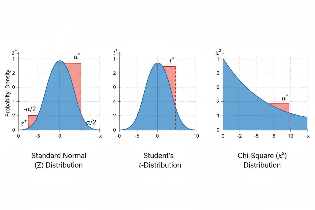
Critical values are cutoff points on a reference probability distribution that separate values considered sufficiently extreme for a statistical procedure from values lying in its central region. They are used in hypothesis tests to define rejection regions and in confidence procedures to determine how far an interval extends from a point estimate. A critical value depends on the chosen significance level or confidence level, whether the procedure is one-sided or two-sided, the reference distribution being used, and—when relevant—the degrees of freedom. For a standard normal distribution, familiar critical values such as 1.645, 1.960, and 2.576 correspond to common confidence levels or tail probabilities. A t critical value additionally depends on degrees of freedom and is generally farther from zero than the corresponding z critical value for finite samples. Chi-square critical values behave differently because the chi-square distribution is nonnegative and asymmetric, so its cutoffs are not simply ± the same number. Selecting the correct critical value is therefore a distributional and inferential decision, not merely a matter of choosing a number from a table.
Critical values form an important part of core statistics and the broader Statistics & Probability framework. Their relationship with the selected confidence level is especially important because changing the desired coverage or significance threshold changes the required cutoff.
What Are Critical Values?
A critical value is a quantile of a probability distribution chosen to leave a specified probability in one or more tails.
Suppose a hypothesis test uses significance level:
α = 0.05
A critical value is selected so that the probability of falling into the rejection region under the null reference distribution equals 0.05.
For a right-tailed test:
P(T ≥ critical value | H₀) = α
For a left-tailed test:
P(T ≤ critical value | H₀) = α
For a symmetric two-tailed test with total significance level α:
P(T ≤ −critical value) + P(T ≥ critical value) = α
when the reference distribution is symmetric around zero.
The observed test statistic is then compared with the appropriate cutoff.
Critical Value vs Test Statistic
The test statistic comes from the sample.
The critical value comes from the reference distribution and the chosen testing rule.
Suppose a z-test has:
Observed z = 2.30
and the right-tailed critical value is:
zcritical = 1.645
Because:
2.30 > 1.645
the test statistic lies in the rejection region.
By contrast, if:
Observed z = 1.20
then:
1.20 < 1.645
so it does not cross the right-tail cutoff.
The critical value does not describe the effect magnitude. It defines a statistical decision boundary under the selected reference model.
Critical Values and Significance Level
The significance level α determines how much reference-distribution probability is allocated to the rejection region.
Common choices include:
α = 0.10
α = 0.05
α = 0.01
A smaller α places the critical boundary farther into the tail.
For a standard normal right-tailed test:
α = 0.10 → zcritical ≈ 1.282
α = 0.05 → zcritical ≈ 1.645
α = 0.01 → zcritical ≈ 2.326
Thus, reducing α makes the rejection criterion more stringent because the observed statistic must be more extreme before H₀ is rejected.
Critical Values and Confidence Level
For many matching two-sided procedures:
Confidence level = 1 − α
Therefore:
90% confidence ↔ α = 0.10
95% confidence ↔ α = 0.05
99% confidence ↔ α = 0.01
The confidence level identifies the long-run coverage target.
For a symmetric two-sided confidence interval, α is divided equally between the two tails:
Tail probability = α/2
For a 95% confidence interval:
α = 0.05
so:
α/2 = 0.025
is placed in each tail.
The standard normal cutoffs are then approximately:
−1.960
and:
+1.960
Quantiles and Critical Values
A critical value is fundamentally a quantile.
If F is the cumulative distribution function of a reference variable T, then a right-tail critical value c satisfying tail probability α obeys:
P(T ≥ c) = α
Equivalently:
P(T ≤ c) = 1 − α
so:
c = F⁻¹(1 − α)
For a two-sided symmetric procedure:
c = F⁻¹(1 − α/2)
This relationship explains how statistical tables and quantile functions generate critical values.
The exact result depends on the chosen distribution.
z Critical Values
A z critical value comes from the standard normal distribution:
Z ~ N(0, 1)
The standard normal distribution has:
Mean = 0
Standard deviation = 1
and is symmetric around zero.
Because of that symmetry, two-sided z critical values occur as:
−z*
and:
+z*
For a two-sided confidence procedure:
z* = Φ⁻¹(1 − α/2)
where Φ is the standard normal CDF.
Common Two-Sided z Critical Values
| Confidence Level | α | α/2 | z* |
|---|---|---|---|
| 80% | 0.20 | 0.10 | 1.282 |
| 90% | 0.10 | 0.05 | 1.645 |
| 95% | 0.05 | 0.025 | 1.960 |
| 98% | 0.02 | 0.01 | 2.326 |
| 99% | 0.01 | 0.005 | 2.576 |
These values are commonly used in normal-based confidence intervals.
For example, a two-sided 95% interval often has the structure:
Estimate ± 1.96 × SE
when a standard normal reference distribution is appropriate.
Common One-Sided z Critical Values
For a one-sided procedure, all of α lies in one tail.
| One-Sided Confidence Level | α | z* |
|---|---|---|
| 90% | 0.10 | 1.282 |
| 95% | 0.05 | 1.645 |
| 99% | 0.01 | 2.326 |
Notice that:
95% one-sided → z* ≈ 1.645
while:
95% two-sided → z* ≈ 1.960
The difference occurs because the two-sided procedure splits α across two tails.
Example: Finding a z Critical Value for a 95% Confidence Interval
Suppose the required confidence level is:
95%
Then:
C = 0.95
so:
α = 1 − 0.95
α = 0.05
For a two-sided interval:
α/2 = 0.025
The upper cutoff must satisfy:
P(Z ≤ z*) = 0.975
The corresponding standard normal quantile is:
z* ≈ 1.960
Therefore, the central region is:
P(−1.960 ≤ Z ≤ 1.960) ≈ 0.95
and the critical values are:
−1.960 and +1.960
Example: z Critical Value for a Right-Tailed Test
Suppose:
H₀: μ = μ₀
H₁: μ > μ₀
with:
α = 0.05
Because the alternative is right-tailed, all rejection probability lies in the upper tail.
We need:
P(Z ≥ zcritical) = 0.05
Therefore:
P(Z ≤ zcritical) = 0.95
and:
zcritical ≈ 1.645
The rejection rule is:
Reject H₀ if zobserved ≥ 1.645
An observed z-statistic of:
z = 1.90
crosses the cutoff.
An observed value of:
z = 1.20
does not.
Left-Tailed z Critical Values
For a left-tailed test with:
α = 0.05
symmetry gives:
zcritical ≈ −1.645
The rejection region is:
Z ≤ −1.645
For:
α = 0.01
the critical value is approximately:
−2.326
The sign therefore depends on which tail contains the rejection region.
The magnitude is determined by the selected tail probability.
Two-Tailed z Tests
Suppose:
H₁: μ ≠ μ₀
and:
α = 0.05
The rejection probability is divided:
α/2 = 0.025
into each tail.
The critical values are:
−1.960
and:
+1.960
The decision rule becomes:
Reject H₀ if z ≤ −1.960 or z ≥ 1.960
Equivalently:
Reject H₀ if |z| ≥ 1.960
This absolute-value form works because the standard normal distribution is symmetric.
When Are z Critical Values Used?
z critical values arise when the reference statistic follows, exactly or approximately, a standard normal distribution.
Examples include certain procedures for:
- population means when the relevant standard error structure is known,
- large-sample proportions,
- large-sample estimator approximations,
- standardized normal test statistics.
However, using a z critical value merely because the sample size “looks large” can be too simplistic.
The appropriate reference distribution depends on the statistical model and estimator.
t Critical Values
A t critical value comes from a Student’s t distribution.
The t distribution is symmetric around zero like the standard normal distribution, but it has heavier tails.
Its exact shape depends on:
degrees of freedom
commonly abbreviated:
df
For a one-sample mean with unknown population standard deviation:
df = n − 1
in the conventional t procedure.
A t critical value can be written:
t* = t₁₋α/₂,df
for a two-sided interval.
Why t Critical Values Depend on Degrees of Freedom
When the population standard deviation σ is unknown, it is often estimated using the sample standard deviation s.
That introduces additional uncertainty.
The t distribution represents this extra uncertainty through heavier tails.
With small df, the tails are substantially heavier than the normal distribution.
Therefore:
t* > z*
for corresponding two-sided confidence levels and finite df.
As degrees of freedom increase, the t distribution approaches the standard normal distribution.
Thus:
t* → z*
as:
df → ∞
Common 95% Two-Sided t Critical Values
For a two-sided 95% procedure:
α = 0.05
and:
α/2 = 0.025
Some common values are:
| df | t* |
|---|---|
| 5 | 2.571 |
| 10 | 2.228 |
| 20 | 2.086 |
| 30 | 2.042 |
| 100 | 1.984 |
| ∞ | 1.960 |
The table illustrates the convergence toward the corresponding normal critical value:
z* ≈ 1.960
as df increases.
Example: Finding a t Critical Value
Suppose a sample has:
n = 11
and a two-sided 95% confidence interval for the population mean is required.
For a conventional one-sample t procedure:
df = n − 1
df = 10
The confidence level is:
0.95
so:
α = 0.05
and:
α/2 = 0.025
The required t quantile is approximately:
t* = 2.228
Therefore, the confidence interval has the form:
x̄ ± 2.228s/√11
The value 1.96 would be too small for this exact t procedure because it ignores the heavier tails associated with estimating σ from a small sample.
One-Sided t Critical Values
A one-sided t procedure places all of α in one tail.
For example, with:
df = 10
and:
α = 0.05
the upper-tail critical value is approximately:
tcritical ≈ 1.812
For a two-sided 95% procedure with the same df:
t* ≈ 2.228
The difference occurs because:
one-sided α = 0.05
uses the 95th percentile, while:
two-sided α = 0.05
uses the 97.5th percentile for the positive cutoff.
Thus, tail structure matters just as much for t distributions as it does for z distributions.
z Critical Values vs t Critical Values
Both z and t distributions are symmetric around zero, but their critical values differ when df is finite.
For a two-sided 95% procedure:
z* ≈ 1.960
while with:
df = 5
we have:
t* ≈ 2.571
and with:
df = 30
we have:
t* ≈ 2.042
The difference becomes smaller as df increases.
This leads to the practical pattern:
Small df → noticeably larger t critical value
Large df → t critical value approaches z critical value
The choice should follow the statistical model rather than selecting whichever cutoff produces a preferred result.
t Critical Values and Confidence Interval Width
Consider:
SE = 4
Using:
z* = 1.960
produces:
Margin of error = 1.960 × 4
= 7.84
Using:
t* = 2.571
produces:
Margin of error = 2.571 × 4
= 10.284
The t-based interval is wider.
This reflects greater uncertainty when the reference procedure requires heavier tails.
As df increases, that difference becomes progressively smaller.
Chi-Square Critical Values
Chi-square critical values come from a chi-square distribution:
Χ² ~ χ²(df)
Unlike z and t distributions, the chi-square distribution is:
- defined only for nonnegative values,
- generally right-skewed,
- dependent strongly on degrees of freedom,
- not symmetric around zero.
Therefore, chi-square critical values do not usually appear as:
±c
Instead, lower-tail and upper-tail quantiles are different positive numbers.
Shape of the Chi-Square Distribution
For a chi-square distribution with ν degrees of freedom:
Mean = ν
Variance = 2ν
The distribution is strongly right-skewed at small df.
As df increases, it becomes less skewed and more nearly symmetric in shape, although it remains nonnegative.
Because the distribution changes substantially with df, the critical value cannot be identified from α alone.
Both:
α
and:
df
are required.
Right-Tail Chi-Square Critical Values
Many chi-square hypothesis tests use an upper-tail rejection region because larger test statistics represent greater disagreement with H₀.
For a right-tailed chi-square test:
P(Χ²df ≥ χ²critical) = α
Some upper-tail α = 0.05 critical values are:
| df | χ² Critical Value |
|---|---|
| 1 | 3.841 |
| 2 | 5.991 |
| 5 | 11.070 |
| 10 | 18.307 |
| 20 | 31.410 |
As df increases, the cutoff also generally increases.
This does not mean larger df automatically provides stronger evidence. The observed statistic must always be evaluated relative to the corresponding reference distribution.
Example: Chi-Square Critical Value for a Test
Suppose a chi-square goodness-of-fit test has:
df = 5
and:
α = 0.05
The right-tail critical value is approximately:
χ²critical = 11.070
The decision rule is:
Reject H₀ if χ²observed ≥ 11.070
If:
χ²observed = 13.2
then:
13.2 > 11.070
and the test statistic falls inside the rejection region.
If:
χ²observed = 7.8
then it does not cross the cutoff.
Chi-Square Critical Values for Variance Intervals
Chi-square distributions are also used when constructing confidence intervals for a population variance under normal-population assumptions.
For a 95% interval:
α = 0.05
so the relevant quantiles are:
χ²0.025,df
and:
χ²0.975,df
These are not symmetric.
For example, with:
df = 10
the relevant chi-square quantiles are approximately:
χ²0.025,10 ≈ 3.247
and:
χ²0.975,10 ≈ 20.483
Notice that these values are not equally spaced around the mean:
10
This asymmetry is one reason variance confidence intervals are themselves asymmetric.
Example: 95% Variance Critical Values
Suppose:
n = 11
so:
df = n − 1 = 10
For a 95% confidence interval:
α = 0.05
and:
α/2 = 0.025
The required chi-square quantiles are approximately:
χ²0.025,10 = 3.247
χ²0.975,10 = 20.483
A population variance interval under the normal model can be written:
[(n − 1)s²/χ²0.975,df, (n − 1)s²/χ²0.025,df]
Notice the apparently reversed placement of the quantiles in the denominators.
The larger chi-square value produces the lower variance endpoint, while the smaller chi-square value produces the upper endpoint.
z, t, and Chi-Square Critical Values Compared
| Feature | z | t | Chi-Square |
|---|---|---|---|
| Distribution | Standard normal | Student’s t | Chi-square |
| Symmetric? | Yes | Yes | No |
| Can be negative? | Yes | Yes | No |
| Depends on df? | No | Yes | Yes |
| Two-sided cutoffs | ±z* | ±t* | Two unequal positive quantiles |
| Common use | Normal-based inference | Means with estimated σ and related procedures | Categorical tests, variance inference |
The correct critical value is determined by the reference distribution associated with the statistic, not merely by the confidence level.
Critical Values and Degrees of Freedom
Degrees of freedom represent the amount of independent information available for estimating variability or determining a reference distribution.
For t procedures, fewer degrees of freedom create heavier tails and larger critical values.
For chi-square distributions, df changes the location, spread, and skewness of the entire distribution.
Examples include:
One-sample t: df = n − 1
Chi-square independence test: df = (r − 1)(c − 1)
Simple goodness-of-fit test: often df = k − 1
although the exact df can change when parameters are estimated from the data.
Degrees of freedom should therefore be calculated from the specific statistical procedure rather than guessed from sample size alone.
One-Tailed vs Two-Tailed Critical Values
The alternative hypothesis determines where the rejection region lies.
For:
H₁: θ > θ₀
the test is right-tailed.
For:
H₁: θ < θ₀
the test is left-tailed.
For:
H₁: θ ≠ θ₀
the test is two-tailed.
At:
α = 0.05
a right-tailed z-test uses:
zcritical ≈ 1.645
A left-tailed test uses:
zcritical ≈ −1.645
A two-tailed test uses:
zcritical ≈ ±1.960
Choosing the number of tails after inspecting the observed data undermines the intended Type I error control.
The test direction should follow the research hypothesis defined in advance.
Critical Values and Rejection Regions
A rejection region contains test-statistic values sufficiently extreme under H₀ according to the chosen α.
For a right-tailed z-test:
Rejection region: z ≥ zcritical
For a left-tailed z-test:
Rejection region: z ≤ zcritical
For a two-tailed z-test:
Rejection region: z ≤ −z* or z ≥ z*
For a typical Pearson chi-square test:
Rejection region: χ² ≥ χ²critical
Critical values therefore translate a probability statement about the reference distribution into a practical decision boundary.
Critical Values and p-Values
Critical-value and p-value methods are two ways of expressing the same hypothesis-testing logic when applied consistently.
The critical-value method asks:
Did the observed statistic cross the rejection boundary?
The p-value method asks:
Is the tail probability associated with the observed statistic less than or equal to α?
For the same test:
Statistic beyond critical value ⇔ p ≤ α
apart from details caused by discrete distributions or particular testing conventions.
For example, if a right-tailed z-test has:
α = 0.05
and:
zcritical = 1.645
then any observed statistic above 1.645 corresponds to a one-sided p-value below 0.05.
A Critical Value Is Not a p-Value
Although they lead to equivalent decisions in compatible procedures, the two quantities are different.
A critical value is a cutoff in units of the reference statistic.
For example:
zcritical = 1.645
A p-value is a probability.
For example:
p = 0.032
The statement:
“The critical value is 0.05”
is generally incorrect when referring to a z, t, or chi-square statistic.
The value:
0.05
is usually α.
The critical value is the reference-distribution quantile corresponding to that α.
Critical Values and Confidence Intervals
Many confidence intervals have the form:
Estimate ± critical value × SE
The selected critical value therefore directly affects interval width.
For a 95% normal-based interval:
z* ≈ 1.960
For a 99% interval:
z* ≈ 2.576
If:
SE = 3
then:
95% margin of error ≈ 1.960 × 3 = 5.88
while:
99% margin of error ≈ 2.576 × 3 = 7.728
The higher-confidence interval is wider because its critical value is larger.
Detailed interval construction belongs with confidence intervals, while the role of the critical value is to set the appropriate reference-distribution cutoff.
Critical Values and Correlation
Formal inference for a correlation coefficient may use a transformed statistic or a t reference distribution.
For testing:
H₀: ρ = 0
a common Pearson-correlation statistic is:
t = r√[(n − 2)/(1 − r²)]
with:
df = n − 2
The observed t value is then compared with t critical values determined by the chosen α, tail structure, and degrees of freedom.
The critical value does not tell us the strength of the correlation.
That role belongs to the estimated coefficient itself.
Critical Values and Covariance
Covariance is primarily a descriptive and mathematical measure of joint variability.
Calculating sample covariance itself does not require a critical value.
Critical values become relevant when performing inference about covariance or related quantities under a specified model.
This distinction is useful:
Descriptive statistic → calculated directly from data
Inferential decision → may require a reference distribution and critical value
A covariance of 20 is not “significant because it exceeds 1.96.” The units and sampling distribution of raw covariance differ from those of a standardized z statistic.
Critical Values and Regression
Regression coefficients are often tested using t statistics or other model-specific test statistics.
In an exponential regression or another regression framework, model parameters may be transformed or estimated using specialized procedures.
A coefficient estimate should not be compared directly with a generic z or t critical value unless it has first been converted into the corresponding test statistic.
For example, a common structure is:
t = estimate/SE(estimate)
under an appropriate null value of zero.
The resulting standardized test statistic, not the raw coefficient alone, is what is compared with the t reference distribution.
Critical Values and Discrete Probability Models
A geometric distribution is a discrete probability distribution, so exact probability calculations may not require z, t, or chi-square critical values.
However, inferential procedures built around geometric or other discrete data can still produce statistics whose reference distributions involve critical values.
This illustrates an important distinction between:
distribution of the original data
and:
reference distribution of a test statistic
They do not have to be the same.
A data set generated from a discrete model can still lead to an approximately normal or chi-square statistic under suitable inferential conditions.
Critical Values and Type I Error
The significance level α is commonly interpreted as the long-run probability of rejecting H₀ when H₀ is true under the specified test procedure.
Critical values are chosen to enforce that rejection probability.
For a right-tailed continuous test:
P(T ≥ c | H₀) = α
where c is the critical value.
Moving c farther into the tail reduces α.
Moving it closer to the center increases α.
The chosen critical boundary therefore directly controls the test’s false-positive probability under its assumptions.
Critical Values and Type II Error
Changing a critical value also affects the probability of failing to reject H₀ when a meaningful alternative is true.
Making α smaller generally moves the rejection boundary farther into the tail.
This reduces Type I error but can increase Type II error for a fixed sample size and effect size.
Statistical testing therefore involves a tradeoff.
Critical values should not be made arbitrarily extreme without considering the consequences for power and the study objective.
Critical Values and Statistical Power
Statistical power is the probability that a test rejects H₀ when a specified alternative is true.
For a fixed sample size and effect:
- moving the critical boundary farther from H₀ usually lowers power,
- increasing sample size can often recover power,
- larger true effects generally make it easier to cross the critical boundary.
Thus, selecting:
α = 0.01
instead of:
α = 0.05
creates a stricter cutoff.
That may reduce false positives but requires stronger evidence to reject H₀.
Critical Values Do Not Measure Effect Size
Suppose a test statistic exceeds its critical value.
That tells us the result crossed the selected statistical threshold.
It does not tell us whether the effect is large enough to matter.
A tiny effect can cross a critical boundary in a very large sample.
A practically important effect can fail to cross it in a small or noisy sample.
Therefore, a hypothesis-test conclusion should often be considered alongside:
- effect estimates,
- uncertainty intervals,
- practical thresholds,
- study design,
- subject-matter importance.
Critical values define inferential thresholds, not substantive importance.
Critical Values Are Not Universal Constants
Some values appear so frequently that they can seem universal.
Examples include:
1.645
1.960
2.576
These are not generic statistical constants.
They are quantiles of the standard normal distribution under particular tail probabilities.
Likewise:
t* = 2.228
is meaningful only when the t distribution and the relevant degrees of freedom are specified.
A chi-square value such as:
3.841
is the upper 5% cutoff only for:
df = 1
Changing df changes the value.
How to Choose the Correct Critical Value
A reliable process involves several steps.
Step 1: Identify the Statistical Procedure
Determine whether the test or interval uses a:
- z distribution,
- t distribution,
- chi-square distribution,
- another reference distribution.
Step 2: Identify α or Confidence Level
For example:
α = 0.05
or:
confidence level = 95%
Step 3: Determine Whether the Procedure Is One-Sided or Two-Sided
For a two-sided procedure:
tail probability = α/2
For a one-sided procedure:
tail probability = α
Step 4: Determine Degrees of Freedom if Required
z critical values do not depend on df.
t and chi-square critical values do.
Step 5: Find the Appropriate Quantile
Use the CDF or quantile function of the reference distribution.
Step 6: Apply the Correct Sign or Tail
For symmetric z and t distributions, left-tail cutoffs are negative and right-tail cutoffs are positive.
For chi-square distributions, cutoffs remain nonnegative.
Example: Choosing Between z and t
Suppose a researcher estimates a population mean from:
n = 16
observations.
The population standard deviation is unknown and estimated using the sample standard deviation.
Under the usual one-sample t framework:
df = 16 − 1
df = 15
For a two-sided 95% procedure, the correct t critical value is approximately:
t* ≈ 2.131
Using:
z* = 1.960
would ignore the extra uncertainty represented by the t distribution.
The difference becomes smaller with larger df, but the reference distribution should be chosen from the model rather than by convenience.
Example: One-Sided vs Two-Sided Critical Values
Suppose:
α = 0.05
For a right-tailed z-test:
zcritical ≈ 1.645
For a two-tailed z-test with the same total α:
zcritical ≈ ±1.960
Why is the two-tailed magnitude larger?
Because the total 5% rejection probability is split:
2.5% left tail
and:
2.5% right tail
The upper boundary therefore has to move farther from zero to leave only 2.5% above it rather than 5%.
Example: Critical Value Decision
Suppose a two-sided t-test has:
df = 20
and:
α = 0.05
The critical values are approximately:
±2.086
Suppose the observed statistic is:
t = −2.40
Because:
−2.40 < −2.086
the statistic lies in the left rejection region.
Therefore:
Reject H₀
under the specified test.
If instead:
t = −1.80
then:
−2.086 < −1.80 < 2.086
so the statistic lies in the nonrejection region.
Example: Chi-Square Decision
Suppose a categorical hypothesis test produces:
χ²observed = 20.0
with:
df = 10
and:
α = 0.05
The upper-tail critical value is:
χ²critical ≈ 18.307
Since:
20.0 > 18.307
the statistic falls in the rejection region.
The data therefore provide sufficient evidence to reject H₀ at the 5% significance level under the assumptions of the chi-square procedure.
This does not mean there is a 95% probability that H₁ is true.
Critical Values From Statistical Tables
Traditional statistical tables organize critical values by:
- significance level,
- tail probability,
- degrees of freedom,
- reference distribution.
For a t table, the rows commonly correspond to df and columns to selected tail probabilities.
For a chi-square table, the same df can have many different lower- or upper-tail critical values.
When reading a table, always verify whether the column heading represents:
upper-tail probability,
lower-tail cumulative probability,
or:
two-sided significance level.
Different textbooks and software can label tables differently.
Critical Values From Software
Statistical software usually obtains critical values from inverse CDF or quantile functions.
Conceptually:
critical value = F⁻¹(probability)
For a two-sided 95% z interval:
z* = Φ⁻¹(0.975)
For a right-tailed chi-square test with:
α = 0.05
the critical value is:
χ²critical = F⁻¹χ²(0.95)
Using software avoids manual table interpolation, but the analyst must still supply the correct probability, distribution, and degrees of freedom.
A perfectly calculated wrong quantile is still the wrong critical value.
Common Critical Value Mistakes
A common mistake is using 1.96 for every 95% procedure. That number is appropriate for a two-sided standard normal procedure, not universally.
Another mistake is forgetting to divide α by two for a two-sided symmetric test or interval.
For:
α = 0.05
the two-sided tail probability is:
0.025 per tail
not 0.05 per tail.
A third error is using the wrong degrees of freedom for a t or chi-square distribution.
It is also incorrect to compare a raw estimate directly with a critical value when the procedure requires a standardized test statistic.
Another frequent mistake is confusing α with the critical value. The significance level may be 0.05, while the corresponding z critical value is 1.645 or 1.960 depending on the test structure.
Analysts can also mistakenly use symmetric ± cutoffs for a chi-square distribution, even though chi-square values cannot be negative.
Finally, selecting a one-tailed test after observing that the data moved in a preferred direction invalidates the intended pre-specified error control.
Critical Values and Statistical Significance
A result is statistically significant at level α when the observed test statistic falls in the rejection region defined by the critical values.
For a two-sided z-test with:
α = 0.05
the rejection regions are:
z ≤ −1.960
or:
z ≥ 1.960
If:
z = 2.40
the result is statistically significant.
If:
z = 1.80
it is not statistically significant at that threshold.
This binary classification depends on α.
The underlying evidence does not suddenly change discontinuously when a statistic moves from 1.95 to 1.97. The cutoff is a decision convention imposed on a continuous measure of evidence.
Critical Values and Practical Interpretation
Critical values are most useful when treated as part of a larger inferential framework.
A rigorous interpretation should consider:
- the observed estimate,
- test statistic,
- uncertainty,
- effect size,
- model assumptions,
- sample size,
- practical consequences.
Crossing a critical value answers a specific statistical question under a specified procedure.
It does not establish that a model is perfectly correct, that an effect is important, or that an observed association is causal.
Frequently Asked Questions About Critical Values
What are critical values?
Critical values are reference-distribution cutoffs that define rejection regions in hypothesis tests or determine the extent of many confidence procedures.
How do you find a critical value?
Identify the reference distribution, α or confidence level, tail structure, and degrees of freedom when applicable, then obtain the corresponding distribution quantile.
What is the z critical value for 95% confidence?
For a conventional two-sided standard normal procedure:
z* ≈ 1.960
What is the z critical value for 90% confidence?
For a conventional two-sided standard normal procedure:
z* ≈ 1.645
What is the z critical value for 99% confidence?
For a conventional two-sided standard normal procedure:
z* ≈ 2.576
What is the one-tailed z critical value for α = 0.05?
For a right-tailed test:
zcritical ≈ 1.645
For a left-tailed test:
zcritical ≈ −1.645
Why is the two-tailed 5% z critical value 1.96 instead of 1.645?
A two-tailed test splits α = 0.05 into 0.025 in each tail. The positive cutoff must therefore leave only 2.5% above it, producing approximately 1.96.
What determines a t critical value?
A t critical value depends on:
- α or confidence level,
- whether the procedure is one-sided or two-sided,
- degrees of freedom.
Why are t critical values larger than z critical values?
For finite degrees of freedom, the t distribution has heavier tails to reflect additional uncertainty from estimating variability. Its cutoffs are therefore farther from zero.
What happens to t critical values as sample size increases?
As degrees of freedom increase, t critical values approach the corresponding z critical values.
What determines a chi-square critical value?
A chi-square critical value depends on the tail probability and degrees of freedom. For two-sided variance procedures, both lower and upper quantiles may be required.
Can a chi-square critical value be negative?
No. The chi-square distribution has support:
x ≥ 0
so all its critical values are nonnegative.
Why are chi-square lower and upper critical values not symmetric?
The chi-square distribution is asymmetric, especially at small degrees of freedom, so equal tail probabilities correspond to unequal distances from the center.
Is a critical value the same as alpha?
No. Alpha is a probability such as 0.05. The critical value is the corresponding cutoff on the reference distribution, such as z = 1.645.
Is a critical value the same as a p-value?
No. A critical value is a reference-distribution threshold. A p-value is a probability calculated from the observed test statistic under H₀.
How are critical values related to confidence intervals?
Many confidence intervals use:
Estimate ± critical value × standard error
A higher confidence level typically requires a larger critical value and therefore a wider interval.
Does exceeding a critical value mean an effect is important?
No. It indicates statistical significance under the selected procedure. Practical importance depends on the effect magnitude, uncertainty, context, and consequences.
Does exceeding a critical value prove the alternative hypothesis?
No. It provides sufficient evidence to reject H₀ according to the chosen test rule. It does not assign certainty or a posterior probability to H₁.
Why do degrees of freedom matter?
Degrees of freedom determine the shape of t and chi-square reference distributions and therefore determine the correct critical cutoff.
Should I use z or t critical values for a mean?
The choice depends on the statistical model and how variability is handled. When the population standard deviation is unknown and estimated from the sample under the conventional normal-theory mean procedure, a t distribution is generally used.
Can the same confidence level have different critical values?
Yes. A 95% confidence level can produce different cutoffs depending on whether the reference distribution is z, t, chi-square, or another distribution, and whether the procedure is one-sided or two-sided.




