


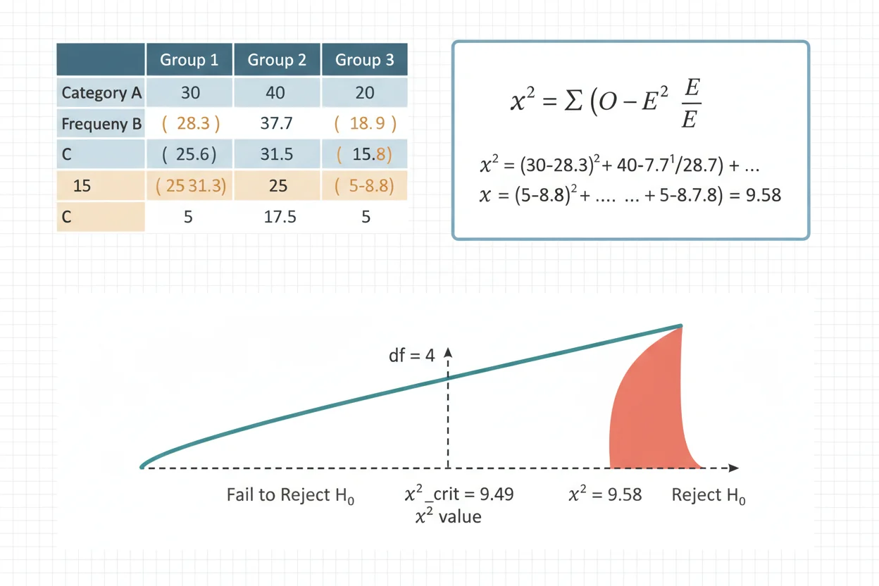
Chi-square is a statistical method used to compare observed categorical frequencies with frequencies expected under a specified null hypothesis. The central chi-square statistic measures how far observed counts deviate from expected counts after scaling each deviation by its expected frequency. A small chi-square statistic indicates that observed and expected frequencies are relatively close, while a large statistic indicates greater disagreement with the null model. Chi-square methods are commonly used for goodness-of-fit questions and for testing whether two categorical variables are associated in a contingency table. The test statistic is nonnegative because every observed-minus-expected difference is squared. Statistical significance is determined by comparing the statistic with an appropriate chi-square reference distribution whose shape depends on the degrees of freedom. A significant result provides evidence against the specified null hypothesis, but it does not measure effect size, establish practical importance, or prove causation.
Chi-square belongs to the inferential methods covered within core statistics and the broader Statistics & Probability framework. It is particularly useful when the data are frequencies in categories rather than continuous measurements or a simple count of successes from a binary process.
What Is Chi-Square?
The term chi-square can refer both to a family of probability distributions and to statistical tests whose test statistics are compared with those distributions.
The chi-square test statistic is commonly written:
χ² = Σ(Oᵢ − Eᵢ)²/Eᵢ
where:
- Oᵢ = observed frequency in category or cell i
- Eᵢ = expected frequency under H₀
- Σ = sum across the relevant categories or cells
The statistic measures discrepancy between what was actually observed and what the null hypothesis predicts.
If:
Oᵢ = Eᵢ
for every category, then every contribution is zero and:
χ² = 0
As the observed frequencies move farther from their expected frequencies, χ² generally becomes larger.
However, the size of χ² cannot be interpreted without considering the degrees of freedom. A value that is unusual with one degree of freedom may be entirely ordinary with many degrees of freedom.
What Does a Chi-Square Test Evaluate?
A chi-square test typically evaluates categorical count data.
Two especially common forms are:
- Chi-square goodness-of-fit test — evaluates whether observed frequencies follow a specified categorical distribution.
- Chi-square test of independence — evaluates whether two categorical variables are statistically associated.
The same general test statistic appears in both settings, but the null hypotheses, expected-frequency calculations, and degrees of freedom differ.
That distinction is essential. “Chi-square” is not one universal procedure that can be applied identically to every table of counts.
Chi-Square Formula
The general Pearson chi-square statistic is:
χ² = Σ(O − E)²/E
For every category or table cell:
- subtract the expected count from the observed count,
- square the difference,
- divide by the expected count,
- add all contributions.
Because squared differences are nonnegative:
χ² ≥ 0
A contribution such as:
(O − E)²/E
becomes larger when observed and expected frequencies differ substantially.
Dividing by E also scales the discrepancy. A difference of 10 observations has a different relative meaning when the expected count is 20 than when it is 2,000.
Why Chi-Square Uses Observed and Expected Counts
A hypothesis test needs a benchmark describing what should occur if H₀ is correct.
For chi-square methods, that benchmark is represented by expected frequencies.
Suppose a fair six-sided die is rolled 120 times. Under the fairness hypothesis, each face has probability:
1/6
The expected count for each face is therefore:
E = 120 × 1/6 = 20
If the observed counts are close to 20 for all six faces, the data are compatible with the fairness model.
If the counts are dramatically uneven, the resulting chi-square statistic becomes larger and the data provide stronger evidence against that model.
Random samples rarely match expected frequencies exactly. The purpose of the test is not to require perfect agreement, but to determine whether the discrepancy is unusually large relative to sampling variation expected under H₀.
Chi-Square Goodness-of-Fit Test
A chi-square goodness-of-fit test compares the observed frequencies of one categorical variable with frequencies predicted by a specified probability model.
Suppose there are k categories with null probabilities:
p₁, p₂, …, pₖ
where:
Σpᵢ = 1
If the total sample size is n, the expected count for category i is:
Eᵢ = npᵢ
The hypotheses are typically:
H₀: The population category probabilities equal the specified probabilities.
H₁: At least one population category probability differs from its specified value.
Notice that H₁ does not necessarily identify which category differs or by how much. It simply states that the complete null distribution does not fit adequately.
Chi-Square Goodness-of-Fit Example
Suppose a six-sided die is rolled 100 times, producing these counts:
| Face | Observed O | Expected E |
|---|---|---|
| 1 | 18 | 16.667 |
| 2 | 16 | 16.667 |
| 3 | 14 | 16.667 |
| 4 | 20 | 16.667 |
| 5 | 17 | 16.667 |
| 6 | 15 | 16.667 |
If the die is fair:
pᵢ = 1/6
for every face.
Therefore:
Eᵢ = 100/6 ≈ 16.667
The chi-square statistic is:
χ² = Σ(Oᵢ − Eᵢ)²/Eᵢ
Substituting all six categories gives:
χ² = (18 − 16.667)²/16.667
- (16 − 16.667)²/16.667
- (14 − 16.667)²/16.667
- (20 − 16.667)²/16.667
- (17 − 16.667)²/16.667
- (15 − 16.667)²/16.667
The result is:
χ² = 1.4
Because there are six categories and the null probabilities were specified in advance:
df = 6 − 1 = 5
The p-value is approximately:
p ≈ 0.9243
At:
α = 0.05
we have:
p > α
so we do not reject H₀.
The sample does not provide evidence that the die’s face probabilities differ from the specified equal-probability model.
This conclusion does not prove that the die is perfectly fair. It means the observed deviations are not unusually large under the stated null model.
Degrees of Freedom for Goodness of Fit
When k category probabilities are completely specified in advance, the usual degrees of freedom are:
df = k − 1
One degree of freedom is lost because the category counts must add to the fixed total n.
If parameters of the expected distribution are estimated from the same data, additional degrees of freedom may need to be subtracted.
A commonly used structure is:
df = k − 1 − m
where m represents the number of independently estimated parameters relevant to the expected probabilities.
The exact degrees-of-freedom calculation therefore depends on how the null model was specified.
Chi-Square Test of Independence
The chi-square test of independence examines whether two categorical variables are associated.
Suppose respondents are classified by:
- membership group: A or B
- preference: Option 1, Option 2, or Option 3
The data form a contingency table.
The hypotheses are:
H₀: The two categorical variables are independent in the population.
H₁: The two categorical variables are associated in the population.
If H₀ is true, the expected frequency of each cell can be calculated from the corresponding row and column totals.
Expected Frequency in a Contingency Table
For cell ij:
Eᵢⱼ = (row total × column total)/grand total
This formula follows from the independence model.
If two events are independent:
P(A ∩ B) = P(A)P(B)
The expected cell frequency reflects this same idea using observed marginal proportions.
Once every expected cell count has been calculated, the statistic becomes:
χ² = ΣΣ(Oᵢⱼ − Eᵢⱼ)²/Eᵢⱼ
where the double sum covers every cell in the table.
Chi-Square Test of Independence Example
Suppose 120 people are divided into two groups, and each chooses one of three options:
| Option 1 | Option 2 | Option 3 | Total | |
|---|---|---|---|---|
| Group A | 30 | 20 | 10 | 60 |
| Group B | 15 | 25 | 20 | 60 |
| Total | 45 | 45 | 30 | 120 |
We want to determine whether group membership and preference are associated.
The hypotheses are:
H₀: Group membership and preference are independent.
H₁: Group membership and preference are associated.
Step 1: Calculate Expected Frequencies
For Group A, Option 1:
E = (60 × 45)/120
E = 22.5
For Group A, Option 2:
E = (60 × 45)/120 = 22.5
For Group A, Option 3:
E = (60 × 30)/120 = 15
Because Group B also has a row total of 60, its expected counts are the same.
The expected table is:
| Option 1 | Option 2 | Option 3 | |
|---|---|---|---|
| Group A | 22.5 | 22.5 | 15 |
| Group B | 22.5 | 22.5 | 15 |
Step 2: Calculate Each Chi-Square Contribution
For Group A, Option 1:
(30 − 22.5)²/22.5 = 2.5
For Group A, Option 2:
(20 − 22.5)²/22.5 ≈ 0.2778
For Group A, Option 3:
(10 − 15)²/15 ≈ 1.6667
For Group B, Option 1:
(15 − 22.5)²/22.5 = 2.5
For Group B, Option 2:
(25 − 22.5)²/22.5 ≈ 0.2778
For Group B, Option 3:
(20 − 15)²/15 ≈ 1.6667
Adding the contributions:
χ² ≈ 8.8889
Step 3: Calculate Degrees of Freedom
For a table with r rows and c columns:
df = (r − 1)(c − 1)
Here:
r = 2
c = 3
Therefore:
df = (2 − 1)(3 − 1)
df = 2
Step 4: Determine the p-Value
For:
χ² ≈ 8.8889
with:
df = 2
the p-value is approximately:
p ≈ 0.0117
At:
α = 0.05
we have:
p < α
so H₀ is rejected.
The data provide evidence of an association between group membership and preference.
They do not, however, demonstrate that group membership causes the preference pattern.
Degrees of Freedom for a Contingency Table
For an r × c contingency table:
df = (r − 1)(c − 1)
For a 2 × 2 table:
df = (2 − 1)(2 − 1) = 1
For a 3 × 4 table:
df = (3 − 1)(4 − 1)
df = 6
Degrees of freedom affect the shape of the chi-square reference distribution and therefore affect both critical values and p-values.
The test statistic cannot be interpreted properly without them.
What Is the Chi-Square Distribution?
The chi-square distribution is a continuous probability distribution defined for nonnegative values.
Its support is:
x ≥ 0
The distribution is generally right-skewed for small degrees of freedom and becomes less skewed as the degrees of freedom increase.
If:
X ~ χ²(ν)
where ν is the degrees of freedom, then:
E(X) = ν
and:
Var(X) = 2ν
The mean of a chi-square distribution therefore equals its degrees of freedom.
The variance is twice the degrees of freedom.
This reference distribution is what allows an observed chi-square statistic to be converted into a tail probability.
Why Chi-Square Tests Use the Right Tail
Large chi-square statistics represent greater discrepancy between observed and expected frequencies.
For Pearson’s chi-square statistic:
χ² = Σ(O − E)²/E
negative and positive deviations are squared, so they both increase the statistic.
Consequently, evidence against H₀ lies in the upper tail of the chi-square distribution.
The p-value is:
P(Χ²df ≥ χ²observed | H₀)
Conceptually, this asks how often a chi-square statistic at least as large as the observed one would arise under the null model.
Interpreting the Chi-Square p-Value
Suppose a test returns:
p = 0.0117
This does not mean there is a 1.17% probability that H₀ is true.
Instead, the p-value describes the probability, assuming H₀ and the model assumptions are true, of obtaining a chi-square statistic at least as large as the observed statistic.
The distinction is the same general frequentist principle that applies to procedures such as ANOVA, although the two tests address different data structures.
The decision framework is commonly:
If p ≤ α, reject H₀.
If p > α, do not reject H₀.
Failing to reject H₀ does not establish that H₀ is exactly true.
Chi-Square and the Confidence Level
The significance level α is related to the corresponding confidence level through:
Confidence level = 1 − α
For example:
α = 0.05
corresponds numerically to:
1 − 0.05 = 0.95
or 95%.
However, hypothesis tests and confidence procedures answer related but distinct inferential questions. A chi-square p-value should not be described as a confidence level, and a 95% confidence level does not mean every statistical conclusion has a 95% probability of being true.
Chi-Square and Confidence Intervals
A chi-square hypothesis test evaluates evidence against a categorical null model, whereas confidence intervals quantify uncertainty around estimated parameters.
When a contingency-table association is statistically significant, an interval for an appropriate effect measure can often provide information that the p-value does not.
A test may answer:
Is there evidence of an association?
An interval may help answer:
What range of effect sizes is compatible with the data under the chosen procedure?
This distinction matters because statistical significance alone does not indicate practical importance.
Statistical Significance vs Practical Significance
With a sufficiently large sample, very small discrepancies between observed and expected frequencies can become statistically significant.
Conversely, an important underlying association may fail to reach statistical significance in a small sample because the test has limited power.
Therefore, a chi-square result should not be evaluated solely by whether:
p < 0.05
The magnitude and practical meaning of the association also matter.
For contingency tables, measures such as Cramér’s V can be used to describe association strength.
For an r × c table:
V = √[χ²/(N × min(r − 1, c − 1))]
where N is the total sample size.
Cramér’s V ranges from 0 to 1, although interpretation depends on table dimensions and substantive context.
A statistically significant association can still have a small effect size.
Assumptions of the Chi-Square Test
Chi-square methods rely on several conditions.
Data Should Be Frequencies
The test generally uses counts of observations in categories.
It should not be applied directly to percentages as though those percentages were raw independent observations.
For example, a table containing:
30, 20, 10
as frequencies differs mathematically from merely entering:
50%, 33.3%, 16.7%
without the underlying sample size.
Expected counts and sampling variability depend on the actual number of observations.
Categories Should Be Mutually Exclusive
Each observation should contribute to the appropriate category or contingency-table cell according to the analysis design.
An individual observation should not be counted repeatedly as independent data unless the statistical method explicitly accounts for that structure.
Observations Should Be Independent
One observation should not determine another observation’s category under the usual Pearson chi-square framework.
Repeated measurements on the same subjects, matched pairs, or clustered observations can violate this condition.
Independence is primarily a property of the sampling and study design.
Expected Counts Should Not Be Too Sparse
The ordinary Pearson chi-square reference distribution is a large-sample approximation.
It works best when expected cell counts are not excessively small.
A value of five is often mentioned as a practical benchmark, but “every expected count must exceed five” is not a universal mathematical rule. Appropriate thresholds and alternatives depend on the table structure and inferential procedure.
When expected frequencies are very sparse, exact, Monte Carlo, permutation, or other specialized methods may be more reliable.
Observed Counts vs Expected Counts
Observed counts come directly from the data.
Expected counts come from H₀.
For the independence test:
Eᵢⱼ = (row total × column total)/N
For a goodness-of-fit test with known category probabilities:
Eᵢ = npᵢ
These quantities should not be confused.
The expected count is not an estimate of what “should have happened” in a deterministic sense. Random variation ensures that observed counts normally differ from expected counts even when the null model is correct.
The test evaluates whether those differences are too large to be reasonably attributed to sampling variation under H₀.
Individual Cell Contributions
Each cell contributes:
(O − E)²/E
to the total statistic.
Examining these contributions can reveal which cells contribute most strongly to a significant result.
In the contingency-table example, the largest contributions came from Option 1 because observed counts of 30 and 15 differed substantially from expected counts of 22.5.
However, raw chi-square contributions should not automatically be treated as independent significance tests.
If detailed cell-level follow-up is needed, standardized residuals and multiple-comparison considerations may be more appropriate.
The omnibus chi-square test answers whether the overall pattern is inconsistent with independence.
Chi-Square Test of Independence vs Goodness of Fit
Although both procedures use:
χ² = Σ(O − E)²/E
their questions differ.
A goodness-of-fit test usually involves one categorical variable and compares its category frequencies with a specified distribution.
A test of independence involves two categorical variables and asks whether their joint frequency pattern is consistent with independence.
For goodness of fit, expected frequencies commonly come from:
Eᵢ = npᵢ
For independence, expected frequencies come from:
Eᵢⱼ = (row total × column total)/N
The formulas look similar because both measure discrepancies between observed and expected frequencies, but the hypotheses must not be confused.
Chi-Square and Binomial Probability
A binary outcome can sometimes be analyzed more directly through binomial probability.
Suppose 7 successes are observed in 10 independent trials and H₀ specifies a particular success probability p. An exact binomial calculation can directly evaluate probabilities under that binary model.
Chi-square methods are especially natural when multiple categorical frequencies are being compared or when a contingency table contains several rows and columns.
For a simple binary problem, a chi-square approximation and an exact binomial procedure may address closely related questions but need not produce identical p-values, especially with small samples.
The data structure and required level of approximation should determine the method.
Chi-Square and the Binomial Distribution
The binomial distribution is a discrete probability model for the number of successes in n independent Bernoulli trials with constant success probability p.
A chi-square reference distribution is continuous and commonly appears as the asymptotic distribution of certain statistical test statistics.
They therefore play very different roles.
The binomial distribution may describe the original data-generating process.
The chi-square distribution may describe the sampling behavior of a test statistic under H₀.
Confusing those roles can lead to incorrect probability calculations.
Chi-Square and Bayes’ Theorem
Bayes’ theorem and chi-square testing belong to different inferential structures.
A traditional chi-square test calculates a p-value under a null hypothesis. It does not assign posterior probabilities to H₀ or H₁.
Bayes’ theorem has the form:
P(A|B) = P(B|A)P(A)/P(B)
and explicitly updates probabilities after observing evidence.
Therefore:
P(data|H₀)
is conceptually different from:
P(H₀|data)
A chi-square p-value cannot be interpreted as the posterior probability that the null hypothesis is true.
Chi-Square Does Not Prove Causation
Suppose a chi-square test finds a statistically significant association between two categorical variables.
That result establishes evidence of association under the test assumptions. It does not establish that one variable causes the other.
Potential explanations may include:
- direct causal effects,
- reverse causation,
- confounding,
- selection effects,
- measurement differences,
- other structural relationships.
Causal conclusions require an appropriate design and substantive reasoning beyond the chi-square statistic.
Chi-Square Does Not Measure Direction
The Pearson chi-square statistic squares every observed-minus-expected difference:
(O − E)²
As a result, the overall χ² statistic does not indicate whether particular observed counts are above or below their expected values.
A large positive deviation and a large negative deviation can both make substantial positive contributions to χ².
To understand the direction of a contingency-table pattern, the original observed and expected values or appropriate residuals must be examined.
What Does χ² = 0 Mean?
If:
χ² = 0
then every observed frequency exactly matches its expected frequency.
That represents perfect sample agreement with the expected counts.
It does not mean the null model has been proven true at the population level.
Samples are finite, and statistical inference concerns uncertainty about the process generating the observations.
In real data, exact agreement is generally unnecessary for a null model to be plausible.
Can a Chi-Square Statistic Be Negative?
No.
Every term has the form:
(O − E)²/E
Expected counts are positive in cells included in the ordinary statistic, and squared differences cannot be negative.
Therefore:
χ² ≥ 0
Any negative result from a supposed Pearson chi-square calculation indicates an arithmetic or implementation error.
Critical Values in Chi-Square Testing
Instead of using a p-value directly, a chi-square test can be expressed through a critical-value decision rule.
For a chosen significance level α and degrees of freedom df, a critical value defines the upper-tail rejection boundary.
The rule is:
Reject H₀ if χ²observed ≥ χ²critical
The p-value and critical-value approaches lead to the same decision when they use the same α and reference distribution.
The exact critical value depends on both:
α
and:
df
so there is no single universal chi-square cutoff.
Why Degrees of Freedom Matter
Chi-square distributions change substantially with degrees of freedom.
With few degrees of freedom, the distribution is strongly right-skewed.
As df increases, its center shifts rightward and its shape becomes less skewed.
Because the reference distribution changes, a raw statistic such as:
χ² = 10
can represent very different evidence depending on df.
That is why results are often reported in a form such as:
χ²(2) = 8.89, p ≈ 0.0117
The degrees of freedom are part of the inferential result rather than an optional detail.
Sample Size and Chi-Square
Sample size affects chi-square testing in two important ways.
First, extremely small samples can produce sparse expected counts, making the usual reference-distribution approximation unreliable.
Second, extremely large samples can make small deviations statistically significant.
Suppose observed proportions differ only slightly from H₀. Multiplying those tiny proportional differences across an enormous sample can still produce a large χ² statistic.
This is another reason effect size and substantive importance should be evaluated alongside statistical significance.
Common Chi-Square Mistakes
A common mistake is using percentages in place of the underlying frequency counts. Chi-square calculations depend on counts and sample size.
Another is using observed frequencies as expected frequencies. Expected counts must be derived from H₀.
A third error is calculating contingency-table expected counts incorrectly. The proper formula is:
Eᵢⱼ = (row total × column total)/grand total
It is also incorrect to interpret a significant chi-square result as proof of causation.
Another frequent mistake is saying that:
p = 0.03
means H₀ has a 3% probability of being true. That is not the frequentist interpretation of a p-value.
Sparse expected cells can also undermine the usual chi-square approximation, so assumptions should be checked before relying on the reported p-value.
Finally, a statistically significant result should not be treated as evidence of a large or practically important association without examining effect size and the actual frequency pattern.
How to Calculate a Chi-Square Test
A general calculation process is:
Step 1: Define the Hypotheses
For goodness of fit, specify the expected category distribution.
For independence, define H₀ as independence between the two categorical variables.
Step 2: Record the Observed Counts
Use actual frequencies rather than percentages alone.
Step 3: Calculate Expected Counts
For goodness of fit:
Eᵢ = npᵢ
For independence:
Eᵢⱼ = (row total × column total)/N
Step 4: Calculate the Test Statistic
χ² = Σ(O − E)²/E
Step 5: Determine Degrees of Freedom
For a simple goodness-of-fit test with completely specified probabilities:
df = k − 1
For an r × c independence table:
df = (r − 1)(c − 1)
Step 6: Obtain the p-Value
Use the upper tail of the chi-square reference distribution.
Step 7: Compare p With α
p ≤ α → reject H₀
p > α → do not reject H₀
Step 8: Interpret the Statistical and Practical Meaning
State what the result says about the categorical pattern while avoiding causal or probability-of-H₀ interpretations that the test does not support.
How to Report a Chi-Square Result
A concise result typically includes:
- the chi-square statistic,
- degrees of freedom,
- sample size when relevant,
- p-value,
- substantive interpretation.
For the independence example:
χ²(2) = 8.89, p ≈ 0.0117
A suitable interpretation is:
The sample provides evidence of an association between group membership and preference.
An unsuitable interpretation would be:
There is a 98.83% probability that the variables are associated.
The chi-square p-value does not provide that posterior probability.
Frequently Asked Questions About Chi-Square
What is chi-square?
Chi-square is a statistical framework commonly used to compare observed categorical frequencies with frequencies expected under a null hypothesis.
What is the chi-square formula?
The Pearson chi-square statistic is:
χ² = Σ(O − E)²/E
where O represents observed frequencies and E represents expected frequencies.
What does a large chi-square value mean?
A large value means observed frequencies differ substantially from expected frequencies relative to the expected counts. Whether it is statistically significant depends on the degrees of freedom and reference distribution.
What does a small chi-square value mean?
A small chi-square statistic indicates relatively close agreement between observed and expected frequencies. It does not prove that H₀ is true.
Can chi-square be negative?
No. Because observed-minus-expected differences are squared, the Pearson chi-square statistic cannot be negative.
What are observed frequencies?
Observed frequencies are the actual category or cell counts recorded in the sample.
What are expected frequencies?
Expected frequencies are the counts predicted under H₀. Their calculation depends on whether the analysis is a goodness-of-fit test, independence test, or another chi-square procedure.
What is the null hypothesis for a chi-square test of independence?
The null hypothesis is:
H₀: The two categorical variables are independent in the population.
The alternative states that they are associated.
What is the null hypothesis for a goodness-of-fit test?
The null hypothesis states that the population category probabilities equal the specified probabilities used to calculate the expected counts.
How do you calculate expected counts in a contingency table?
For each cell:
Eᵢⱼ = (row total × column total)/grand total
How are chi-square degrees of freedom calculated?
For an r × c independence table:
df = (r − 1)(c − 1)
For a simple goodness-of-fit test with k completely specified categories:
df = k − 1
with further adjustments possible when parameters are estimated from the data.
Does p < 0.05 mean the null hypothesis is probably false?
No. It means the observed statistic is sufficiently unusual under H₀ to cross the chosen α = 0.05 rejection threshold. It does not calculate P(H₀|data).
Does a significant chi-square result prove causation?
No. It provides evidence of an association or lack of fit, depending on the test. Causal conclusions require additional design and substantive justification.
What happens when expected counts are very small?
The usual chi-square approximation may become unreliable. Exact, simulation-based, permutation, or other specialized methods may be more appropriate depending on the table and research question.
Is chi-square the same as binomial probability?
No. Binomial probability models the count of successes in repeated binary trials. Chi-square procedures generally compare observed categorical frequencies with frequencies expected under a null model.
Is chi-square the same as ANOVA?
No. ANOVA usually compares means of quantitative outcomes across groups, whereas chi-square methods primarily analyze categorical frequencies.
What is the difference between chi-square significance and effect size?
Statistical significance evaluates evidence against H₀. Effect size describes the magnitude of the departure or association. A result can be statistically significant while having little practical importance.




