


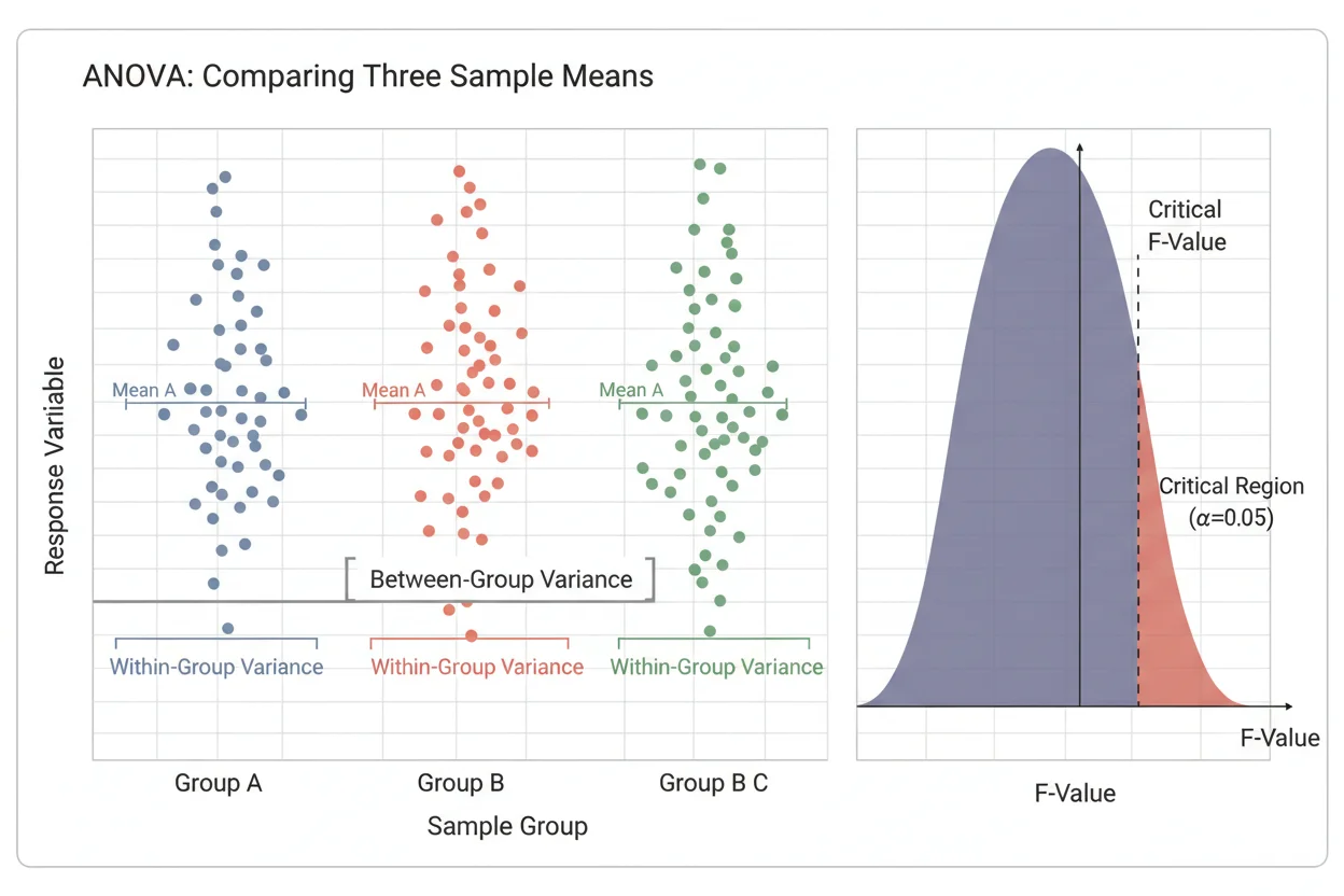
ANOVA, short for analysis of variance, is a statistical method used to test whether the means of three or more groups differ by more than would reasonably be expected from random variation alone. Rather than comparing every pair of group means separately, ANOVA evaluates all groups within one overall hypothesis test. The method works by separating total variability into variation between groups and variation within groups, then comparing those two components through an F statistic. A large F statistic indicates that group means are separated substantially relative to the ordinary variation observed inside the groups. However, a statistically significant ANOVA result does not by itself identify which specific groups differ. It also does not establish that the grouping variable caused the observed difference. ANOVA is therefore most useful when its hypotheses, assumptions, effect size, and any necessary follow-up comparisons are interpreted together.
Within core statistics, ANOVA is one of the standard inferential procedures for comparing group means, while the broader Statistics & Probability framework also includes probability models, estimation methods, categorical tests, and other forms of statistical inference.
What Is ANOVA?
ANOVA tests whether several population means can reasonably be treated as equal based on sample data.
For a one-way ANOVA with k groups, the hypotheses are:
H₀: μ₁ = μ₂ = μ₃ = … = μₖ
H₁: Not all population means are equal.
The null hypothesis H₀ states that every group has the same population mean. The alternative hypothesis H₁ does not necessarily state that every group differs from every other group. It means only that at least one population mean differs from another.
Suppose a researcher measures the same continuous outcome for three independent groups. If the sample means differ slightly, the differences may simply reflect ordinary sampling variation. ANOVA asks whether the observed separation between those group means is large enough, relative to variability within the groups, to provide evidence against H₀.
That logic distinguishes ANOVA from probability-updating methods such as Bayes’ theorem. A frequentist ANOVA p-value measures how incompatible the observed test statistic is with H₀ under the reference model; it is not the probability that H₀ is true.
Why ANOVA Uses Variance to Compare Means
The name analysis of variance can seem unusual because the primary question concerns means, not merely variances. The reason is that differences among means create a particular form of variability.
If all group means are close together, between-group variation will be small. If the means are widely separated, between-group variation will be larger. ANOVA compares this between-group variation with the natural variation found among observations belonging to the same group.
The basic logic is:
F = between-group variance estimate / within-group variance estimate
Under H₀, both parts estimate the same underlying error variance, apart from random sampling fluctuations. Consequently, F values near 1 are generally consistent with little systematic separation among the group means. Larger F values provide increasing evidence that the groups are not all centered at the same population mean.
The exact significance of an F value depends on its degrees of freedom, so an F statistic should never be interpreted from its magnitude alone.
One-Way ANOVA
A one-way ANOVA examines one categorical explanatory factor with two or more levels and one quantitative response variable.
For example, suppose students are assigned to three teaching methods and later take the same examination. The factor is teaching method, with three levels, and the response is examination score.
A one-way ANOVA asks whether the population mean score is the same for all three teaching methods.
Although ANOVA can technically be performed with two groups, an independent-samples t-test usually provides a more familiar equivalent analysis in that special case. ANOVA becomes particularly useful when three or more groups must be evaluated simultaneously.
ANOVA Formula
Assume there are k groups and N observations in total.
Let:
- xᵢⱼ = observation i in group j
- x̄ⱼ = sample mean of group j
- x̄G = grand mean across all observations
- nⱼ = sample size of group j
- k = number of groups
- N = total sample size
The total variability is divided into between-group and within-group sums of squares.
Between-Group Sum of Squares
The between-group sum of squares measures how far each group mean lies from the grand mean, weighted by the size of that group.
SSbetween = Σ nⱼ(x̄ⱼ − x̄G)²
If all group means are close to the grand mean, SSbetween will be small. If several group means lie far from the grand mean, it will be larger.
Within-Group Sum of Squares
The within-group sum of squares measures variability of individual observations around their own group means.
SSwithin = ΣΣ(xᵢⱼ − x̄ⱼ)²
This quantity represents variation that remains inside the groups rather than variation explained by differences among their sample means.
Total Sum of Squares
Total variation around the grand mean is:
SStotal = ΣΣ(xᵢⱼ − x̄G)²
For an ordinary one-way ANOVA:
SStotal = SSbetween + SSwithin
This decomposition is one of the central mathematical ideas behind ANOVA.
ANOVA Degrees of Freedom
Sums of squares must be converted into mean squares before calculating the F statistic.
For k groups:
dfbetween = k − 1
For N total observations:
dfwithin = N − k
The total degrees of freedom are:
dftotal = N − 1
These relationships satisfy:
dftotal = dfbetween + dfwithin
The corresponding mean squares are:
MSbetween = SSbetween/(k − 1)
MSwithin = SSwithin/(N − k)
Finally:
F = MSbetween/MSwithin
Under H₀ and the classical ANOVA assumptions, the F statistic follows an F distribution with:
df₁ = k − 1
df₂ = N − k
The numerator and denominator degrees of freedom determine the appropriate reference distribution used to calculate the p-value.
ANOVA Example
Consider three independent groups with four observations each:
| Group A | Group B | Group C |
|---|---|---|
| 8 | 5 | 10 |
| 9 | 4 | 9 |
| 6 | 6 | 11 |
| 7 | 5 | 10 |
The group means are:
x̄A = (8 + 9 + 6 + 7)/4 = 7.5
x̄B = (5 + 4 + 6 + 5)/4 = 5
x̄C = (10 + 9 + 11 + 10)/4 = 10
There are 12 observations, so the grand mean is:
x̄G = 90/12 = 7.5
Step 1: Calculate SSbetween
Each group contains four observations.
SSbetween = 4(7.5 − 7.5)² + 4(5 − 7.5)² + 4(10 − 7.5)²
SSbetween = 0 + 25 + 25
SSbetween = 50
Step 2: Calculate SSwithin
For Group A:
SSA = (8 − 7.5)² + (9 − 7.5)² + (6 − 7.5)² + (7 − 7.5)²
SSA = 0.25 + 2.25 + 2.25 + 0.25 = 5
For Group B:
SSB = (5 − 5)² + (4 − 5)² + (6 − 5)² + (5 − 5)²
SSB = 0 + 1 + 1 + 0 = 2
For Group C:
SSC = (10 − 10)² + (9 − 10)² + (11 − 10)² + (10 − 10)²
SSC = 0 + 1 + 1 + 0 = 2
Therefore:
SSwithin = 5 + 2 + 2 = 9
Total variation is:
SStotal = 50 + 9 = 59
Step 3: Calculate Degrees of Freedom
There are k = 3 groups and N = 12 observations.
dfbetween = 3 − 1 = 2
dfwithin = 12 − 3 = 9
dftotal = 12 − 1 = 11
Step 4: Calculate Mean Squares
MSbetween = 50/2 = 25
MSwithin = 9/9 = 1
Step 5: Calculate the F Statistic
F = 25/1 = 25
The ANOVA result is therefore:
F(2, 9) = 25
For this F statistic, the p-value is approximately:
p ≈ 0.00021
At a significance level of α = 0.05, p < α, so H₀ is rejected. The data provide strong evidence that the three population means are not all equal.
This conclusion does not establish that every pair of group means differs, nor does it indicate which differences are responsible. Post-hoc comparisons or planned contrasts are needed when the specific group differences matter.
The ANOVA Table
The calculations are commonly organized in an ANOVA table:
| Source | Sum of Squares | df | Mean Square | F |
|---|---|---|---|---|
| Between groups | 50 | 2 | 25 | 25 |
| Within groups | 9 | 9 | 1 | — |
| Total | 59 | 11 | — | — |
The p-value is obtained by comparing the observed F = 25 with an F distribution having 2 numerator and 9 denominator degrees of freedom.
How to Interpret an ANOVA p-Value
The p-value is calculated under the assumption that H₀ is true. It represents the probability, under the null model and its assumptions, of obtaining an F statistic at least as extreme as the observed value.
A small p-value indicates that the observed ratio of between-group to within-group variation would be unusual if all population means were equal.
It does not mean:
“There is a p × 100% probability that H₀ is true.”
Nor does p < 0.05 prove that the alternative hypothesis is correct with 95% probability.
That distinction is essential. ANOVA belongs to a frequentist hypothesis-testing framework, whereas posterior probabilities require a different inferential framework.
Significance Level and ANOVA Decision Rule
Before examining the result, a significance level α is normally selected. A common choice is 0.05, although the appropriate value depends on the consequences of false-positive and false-negative conclusions.
The decision rule is:
If p ≤ α, reject H₀.
If p > α, do not reject H₀.
Failing to reject H₀ does not prove that all population means are identical. It indicates that the data do not provide sufficiently strong evidence of a difference under the chosen testing procedure.
Statistical Significance vs Practical Significance
A statistically significant ANOVA result says something about evidence against equal population means. It does not automatically tell you whether the difference is large enough to matter in practice.
Large samples can detect very small effects, while small samples can fail to detect effects that may be practically meaningful. Therefore, an ANOVA result should often be considered alongside effect sizes and confidence intervals.
In the numerical example:
η² = SSbetween/SStotal
η² = 50/59 ≈ 0.847
This means that about 84.7% of the observed sample variation is associated with differences among the three groups in this deliberately simple data set.
Effect-size interpretation must depend on the subject area rather than on a universal rule that labels every numerical value as small, medium, or large.
Assumptions of Classical One-Way ANOVA
The validity of the standard ANOVA F test depends on several conditions.
Independent Observations
Observations should be independent within and across groups according to the study design. Repeated measurements from the same individual, matched observations, clustered samples, or other dependencies require methods that explicitly account for those relationships.
Independence is primarily a design issue. It cannot usually be repaired simply by inspecting the observed data.
Approximately Normal Errors Within Groups
Classical ANOVA assumes that the model errors are normally distributed within each population group.
The method is often reasonably robust to moderate non-normality when sample sizes are adequate and the groups are reasonably balanced. Severe skewness, extreme outliers, or very small samples can make the approximation unreliable.
Equal Population Variances
Standard one-way ANOVA assumes:
σ₁² = σ₂² = … = σₖ²
This is called homogeneity of variance or homoscedasticity.
Unequal variances become particularly problematic when group sample sizes are also unequal. Welch’s ANOVA is often more appropriate when population variances cannot reasonably be treated as equal.
Quantitative Response Variable
Classical ANOVA is designed for a quantitative dependent variable.
When the outcome is a count of successes or failures rather than a continuous measurement, probability models such as the binomial distribution and calculations involving binomial probability may better match the data-generating process.
For categorical frequency data, a procedure such as a chi-square test often addresses a different and more appropriate statistical question.
What Happens After a Significant ANOVA?
A significant omnibus ANOVA establishes evidence that at least one population mean differs, but it does not isolate the difference.
Suppose four treatment groups produce a significant F test. Possible patterns include one unusual group and three similar groups, two clusters of similar groups, or several distinct means.
Post-hoc procedures can compare group pairs while controlling the increased false-positive risk created by multiple comparisons. Planned contrasts can instead test specific comparisons defined in advance.
The choice should follow the scientific question rather than simply testing every possible pair because the omnibus ANOVA happened to be significant.
Why Not Perform Many t-Tests Instead?
If three groups are compared pairwise, there are three comparisons. With five groups, there are ten. As the number of separate tests increases, the probability of obtaining at least one false-positive result across the collection also increases when no adjustment is made.
One-way ANOVA first evaluates a single omnibus null hypothesis about all group means. If evidence against that hypothesis is found, appropriately controlled follow-up comparisons can then investigate the pattern.
This is one of the main reasons ANOVA is preferable to an uncontrolled collection of independent pairwise tests.
ANOVA and Causation
ANOVA can show an association between group membership and the response variable, but the statistical test itself does not establish causation.
Causal interpretation depends on study design, random assignment, confounding, measurement quality, selection effects, and other substantive considerations. An observational ANOVA can detect mean differences while leaving the reason for those differences unresolved.
Randomized experiments can support stronger causal conclusions when the design and implementation justify them.
ANOVA vs Chi-Square
ANOVA and chi-square tests can both compare patterns across groups, but they typically apply to different types of outcomes.
ANOVA generally analyzes a quantitative response and tests differences among population means. A chi-square procedure generally analyzes counts in categories and compares observed frequencies with expected frequencies or assesses association between categorical variables.
Using ANOVA for purely categorical frequency data simply because several groups are present confuses the statistical question with the number of groups.
ANOVA vs Probability Models
ANOVA is an inferential model for comparing means, whereas probability distributions describe the probabilities associated with random variables.
For example, the binomial model concerns the number of successes in a fixed number of independent Bernoulli trials with constant success probability. That is fundamentally different from asking whether several groups have equal continuous-outcome means.
Likewise, Bayes’ theorem describes how conditional probabilities are updated when new evidence is observed. It should not be used interchangeably with the p-value from an ANOVA test.
Common ANOVA Mistakes
One common mistake is interpreting a significant omnibus test as evidence that all groups differ. ANOVA only indicates that the population means are not all equal.
Another is treating p < 0.05 as a measure of effect magnitude. A very small p-value can occur with a tiny effect in a sufficiently large sample.
A third mistake is ignoring the study design. Standard one-way ANOVA is inappropriate when observations are paired, repeatedly measured, or clustered in a way that violates independence.
Analysts can also obtain misleading results by overlooking extreme outliers, severely unequal variances, or strong distributional problems, particularly with small or highly unbalanced samples.
Finally, statistical significance should not replace subject-matter judgment. Estimates, uncertainty, effect size, and practical consequences remain important even when the ANOVA test rejects H₀.
Frequently Asked Questions About ANOVA
What does ANOVA stand for?
ANOVA stands for analysis of variance. It uses variance components to test whether several population means are all equal.
What is the null hypothesis in ANOVA?
For a one-way ANOVA with k groups:
H₀: μ₁ = μ₂ = … = μₖ
The alternative states that not all population means are equal.
What does a significant ANOVA mean?
A significant ANOVA provides evidence that at least one population mean differs from another. It does not identify the specific pair or pairs responsible for the result.
What is the ANOVA F statistic?
The F statistic is:
F = MSbetween/MSwithin
It compares variability attributable to differences among group means with variability observed within the groups.
Is a larger F statistic always statistically significant?
No. Statistical significance depends on the F value together with the numerator and denominator degrees of freedom. The same F value can correspond to different p-values under different F distributions.
What does p < 0.05 mean in ANOVA?
If α = 0.05, p < 0.05 means the observed F statistic or a more extreme one would be sufficiently unusual under H₀ to meet the chosen rejection criterion. It does not mean there is less than a 5% probability that H₀ is true.
Does ANOVA show which groups are different?
Not by itself. A significant omnibus ANOVA indicates that the means are not all equal. Follow-up contrasts or multiple-comparison procedures are required to determine where the differences lie.
Can ANOVA be used for two groups?
Yes. A one-way ANOVA with two independent groups is mathematically related to the corresponding independent-samples t-test, with F = t² under the usual equal-variance setup. For two groups, the t-test is often easier to interpret.
What if the group variances are unequal?
When heteroscedasticity is substantial, especially with unequal group sizes, Welch’s ANOVA may be preferable to the classical equal-variance test.
Does ANOVA prove causation?
No. The test detects evidence of mean differences. Causal interpretation requires an appropriate research design and control of competing explanations.




