


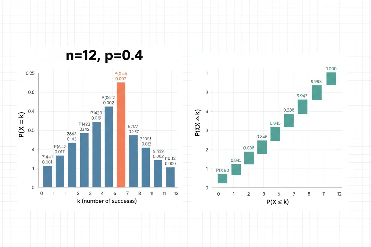
The binomial distribution is a discrete probability distribution that models the number of successes observed in a fixed number of independent trials when every trial has the same probability of success. It is appropriate for situations such as counting how many defective items appear in a fixed sample, how many customers respond to an offer, or how many successes occur in repeated yes-or-no experiments. A binomial random variable is determined by two parameters: the number of trials n and the probability of success p on each trial. Its probability mass function, or PMF, gives the probability of exactly x successes. Its cumulative distribution function, or CDF, gives the probability of obtaining at most a specified number of successes. Because the binomial distribution is discrete, probabilities are assigned to individual integer values rather than to intervals through a probability density function. The model is simple but only valid when its assumptions about the number of trials, binary outcomes, independence, and constant success probability are reasonable.
The binomial distribution is a core discrete model within core statistics and the wider Statistics & Probability framework. Its PMF describes the full probability pattern, while individual calculations involving exact, cumulative, or complementary events can be handled in more detail through binomial probability.
What Is the Binomial Distribution?
A binomial distribution describes a random variable X representing the number of successes in n trials.
It is written as:
X ~ Bin(n, p)
where:
- n = fixed number of trials
- p = probability of success on each trial
- 1 − p = probability of failure on each trial
- X = number of successes
The possible values of X are:
X ∈ {0, 1, 2, …, n}
If n = 8, for example, the number of successes can only be 0, 1, 2, …, 8. Values such as 3.5 or 9 are impossible.
The word success does not necessarily describe a desirable outcome. In probability theory, success simply means the outcome being counted. If a manufacturer is counting defective products, a defective product can be defined as a “success” for purposes of the model.
Conditions for a Binomial Distribution
A random process follows a binomial distribution when four main conditions are satisfied.
Fixed Number of Trials
The number of trials n must be determined in advance.
If a process continues until the first success occurs, the number of trials is not fixed, so an ordinary binomial model is not the appropriate distribution.
Two Outcomes Per Trial
Each trial must be classified into one of two mutually exclusive categories.
These are conventionally called:
Success
and:
Failure
The original experiment can sometimes have more than two physical outcomes as long as they are meaningfully collapsed into two categories for the question being analyzed.
Constant Probability of Success
The success probability p must remain the same on every trial.
If:
P(success on trial 1) = 0.30
then a standard binomial model requires:
P(success on trial 2) = 0.30
and similarly for every other trial.
If the probability changes materially from one trial to another, the ordinary binomial distribution no longer describes the process exactly.
Independent Trials
The outcome of one trial should not change the probability distribution of another trial.
Independence is essential because the binomial PMF multiplies trial probabilities under that assumption.
Sampling without replacement from a small finite population can violate independence because each observation changes the composition of the remaining population. When the sampled fraction is very small relative to the population, the binomial model may sometimes be a useful approximation, but the exact model is different.
Parameters of the Binomial Distribution
The binomial distribution has two parameters:
n = number of trials
p = probability of success per trial
Once n and p are known, the entire distribution is determined.
For example:
X ~ Bin(20, 0.4)
means that X counts successes across 20 trials, each having success probability 0.4.
The failure probability is:
q = 1 − p
so in this case:
q = 1 − 0.4 = 0.6
Some formulas use q for convenience, although p and 1 − p contain the same information.
Binomial Distribution PMF
Because the binomial distribution is discrete, it uses a probability mass function, or PMF.
The PMF gives the probability of exactly x successes:
P(X = x) = C(n, x)pˣ(1 − p)ⁿ⁻ˣ
where:
C(n, x) = n!/[x!(n − x)!]
and:
x = 0, 1, 2, …, n
The combination term C(n, x) counts the number of different ways x successes can occur among n trials.
The term:
pˣ
is the probability contribution from x successes.
The term:
(1 − p)ⁿ⁻ˣ
is the probability contribution from the remaining n − x failures.
Multiplying these parts gives the probability of exactly x successes.
Why the Combination Term Appears
Suppose four trials contain exactly two successes.
One possible sequence is:
S S F F
but two successes can occur in several arrangements:
S F S F
F S S F
F F S S
and others.
Each sequence containing two successes and two failures has the same probability when p is constant and trials are independent.
The number of such sequences is:
C(4, 2) = 6
The binomial PMF therefore multiplies the probability of one particular success-failure arrangement by the number of arrangements that contain exactly x successes.
That combinatorial structure is what distinguishes the probability of exactly x successes from the probability of one particular sequence.
Binomial Distribution PMF Example
Suppose:
X ~ Bin(10, 0.3)
This means there are 10 independent trials and each trial has a 30% probability of success.
To find the probability of exactly four successes:
P(X = 4) = C(10, 4)(0.3)⁴(0.7)⁶
First:
C(10, 4) = 210
Therefore:
P(X = 4) = 210(0.3)⁴(0.7)⁶
P(X = 4) ≈ 0.2001
So the probability of exactly four successes is approximately:
20.01%
This is one value of the PMF. Repeating the calculation for x = 0 through x = 10 produces the complete binomial distribution.
Detailed methods for exact, “at least,” “at most,” and range calculations belong naturally with binomial probability, while the focus here is the structure of the distribution itself.
What Is the Binomial CDF?
The cumulative distribution function, or CDF, gives the probability that X is less than or equal to a specified value.
For a binomial random variable:
F(x) = P(X ≤ x)
For an integer x between 0 and n:
F(x) = Σₖ₌₀ˣ C(n, k)pᵏ(1 − p)ⁿ⁻ᵏ
The CDF therefore adds PMF values from zero through x.
For example:
F(4) = P(X ≤ 4)
means:
P(X ≤ 4) = P(X = 0) + P(X = 1) + P(X = 2) + P(X = 3) + P(X = 4)
Unlike the PMF, which assigns probability to a particular value, the CDF accumulates probability from the lower end of the distribution.
Binomial Distribution CDF Example
Continue with:
X ~ Bin(10, 0.3)
Suppose we want:
P(X ≤ 4)
The CDF calculation is:
P(X ≤ 4) = Σₖ₌₀⁴ C(10, k)(0.3)ᵏ(0.7)¹⁰⁻ᵏ
Evaluating the five PMF terms gives:
P(X ≤ 4) ≈ 0.8497
Therefore, the probability of observing four or fewer successes is approximately:
84.97%
The CDF at x = 4 is consequently:
F(4) ≈ 0.8497
Because X is discrete, the binomial CDF is a step function rather than a smooth curve.
PMF vs CDF
The PMF and CDF describe the same binomial distribution from different perspectives.
| Function | Meaning | Example |
|---|---|---|
| PMF | Probability of one exact value | P(X = 4) |
| CDF | Probability up to and including a value | P(X ≤ 4) |
| PMF notation | P(X = x) | P(X = 4) |
| CDF notation | F(x) = P(X ≤ x) | F(4) |
For:
X ~ Bin(10, 0.3)
we found:
P(X = 4) ≈ 0.2001
but:
P(X ≤ 4) ≈ 0.8497
These quantities are different because the CDF includes the probabilities of 0, 1, 2, 3, and 4 successes, while the PMF includes only exactly four successes.
Why the Binomial Distribution Has a PMF, Not a PDF
A probability density function, or PDF, is associated with continuous random variables.
The binomial distribution is discrete. Its possible values are countable integers:
0, 1, 2, …, n
An individual value can therefore have positive probability:
P(X = 4) > 0
That is why the appropriate function is a probability mass function.
For a continuous random variable, an individual point normally has probability zero, and probabilities are obtained by integrating a density over an interval. These are fundamentally different mathematical structures.
Using “PDF” for the binomial distribution is therefore technically incorrect when referring to its point probabilities.
Mean of the Binomial Distribution
If:
X ~ Bin(n, p)
then the expected value is:
μ = E(X) = np
This represents the long-run average number of successes across repeated sets of n trials.
Suppose:
X ~ Bin(100, 0.2)
Then:
μ = 100 × 0.2 = 20
The expected number of successes is 20.
This does not mean every sample will contain exactly 20 successes. Individual observations of X can vary around the mean.
Variance of the Binomial Distribution
The variance is:
σ² = Var(X) = np(1 − p)
Using:
X ~ Bin(100, 0.2)
we obtain:
σ² = 100 × 0.2 × 0.8
σ² = 16
The standard deviation is:
σ = √[np(1 − p)]
Therefore:
σ = √16 = 4
So this distribution has:
Mean = 20
Variance = 16
Standard deviation = 4
The variance quantifies the spread of the count of successes around its expected value.
Why Variance Depends on p
The variance:
np(1 − p)
is largest, for fixed n, when p = 0.5.
When p is close to 0, successes are rare, so the count tends to stay near zero.
When p is close to 1, failures are rare, so the count tends to remain near n.
At p = 0.5, neither outcome dominates strongly, creating greater uncertainty about the exact number of successes.
For fixed n:
Maximum variance = n/4
which occurs at:
p = 0.5
Shape of the Binomial Distribution
The shape depends primarily on n and p.
When p = 0.5
A binomial distribution is symmetric around its center when:
p = 0.5
For example:
X ~ Bin(20, 0.5)
has mean:
μ = 10
and probabilities are symmetric around 10.
When p < 0.5
When p is substantially below 0.5, successes are relatively uncommon and the distribution is generally right-skewed.
For example:
X ~ Bin(20, 0.1)
places much of its probability near smaller counts and has a longer tail toward larger values.
When p > 0.5
When p is substantially above 0.5, the distribution is generally left-skewed.
For example:
X ~ Bin(20, 0.9)
places much of its probability near the upper end of the possible success counts.
As n becomes larger and p remains away from 0 and 1, the binomial distribution often becomes increasingly bell-shaped.
Mode of the Binomial Distribution
The mode is the most probable number of successes.
For a binomial random variable, the mode is generally related to:
(n + 1)p
If (n + 1)p is not an integer, the unique mode is:
floor[(n + 1)p]
If (n + 1)p is an integer m, there are two adjacent modes:
m − 1
and:
m
For example, if:
n = 10
p = 0.3
then:
(n + 1)p = 11 × 0.3 = 3.3
so the mode is:
floor(3.3) = 3
The most probable count is therefore three successes.
Support of the Binomial Distribution
The support is the set of values the random variable can take.
For:
X ~ Bin(n, p)
the support is:
{0, 1, 2, …, n}
When 0 < p < 1, every integer in that set has positive probability.
At boundary cases, the distribution becomes degenerate.
If:
p = 0
then:
P(X = 0) = 1
If:
p = 1
then:
P(X = n) = 1
These are still mathematically valid special cases of the binomial distribution, although there is no randomness in the number of successes.
Complementary Probabilities
The CDF is also useful for complementary events.
For example:
P(X > x) = 1 − P(X ≤ x)
Therefore:
P(X > x) = 1 − F(x)
Similarly, because X takes integer values:
P(X ≥ x) = 1 − P(X ≤ x − 1)
This distinction is important.
For a discrete random variable:
P(X > 4)
and:
P(X ≥ 4)
are not the same event.
The first excludes four successes, while the second includes it.
Careful treatment of inclusive and exclusive endpoints prevents many common binomial probability errors.
Probability Over an Interval
If a binomial random variable must fall between two integer values a and b, inclusive:
P(a ≤ X ≤ b)
the CDF can be used as:
P(a ≤ X ≤ b) = F(b) − F(a − 1)
For example:
P(3 ≤ X ≤ 6) = F(6) − F(2)
This identity follows because F(6) includes all outcomes from 0 through 6, while F(2) removes outcomes from 0 through 2.
The remaining probability corresponds exactly to 3, 4, 5, or 6 successes.
Binomial Distribution and Bernoulli Trials
A single trial with two outcomes and success probability p follows a Bernoulli distribution.
A binomial random variable is the sum of n independent Bernoulli random variables with the same p.
If:
Yᵢ = 1 for success
and:
Yᵢ = 0 for failure
then:
X = Y₁ + Y₂ + … + Yₙ
and:
X ~ Bin(n, p)
provided the Yᵢ variables are independent and share the same probability p.
This representation also explains the mean:
E(X) = np
because the expected value of each Bernoulli trial is p.
It likewise leads to:
Var(X) = np(1 − p)
because independent variances add.
Binomial Distribution and Bayes’ Theorem
The Bayes’ theorem formula and the binomial distribution serve different purposes.
The binomial distribution calculates the probability of observing a particular number of successes when n and p are specified.
Bayes’ theorem reverses or updates conditional probabilities after evidence is observed.
The two can nevertheless appear together.
Suppose two competing hypotheses imply different success probabilities. A binomial distribution can provide:
P(data|H₁)
and:
P(data|H₂)
for the observed count.
Those likelihoods can then contribute to a Bayesian update.
The binomial model describes the sampling probability of the count; Bayes’ theorem specifies how that evidence changes probability assigned to competing hypotheses.
Binomial Distribution vs ANOVA
The binomial distribution is also fundamentally different from ANOVA.
ANOVA is typically used to compare population means across groups when the response is quantitative and its model assumptions are appropriate.
The binomial distribution instead describes a count of successes across binary trials.
For example, comparing average examination scores across three teaching methods is an ANOVA-type question. Counting how many students out of 20 pass under a fixed success probability is a binomial-type model.
The number of groups alone does not determine the correct method. The response variable and the data-generating process are more important.
Binomial Distribution vs Chi-Square
A chi-square test often analyzes observed category counts and compares them with expected frequencies.
The binomial distribution instead provides a probability model for the number of successes in repeated binary trials.
A binomial model may sometimes be used to derive expected probabilities or test statistics, but a chi-square procedure and a binomial distribution do not answer the same question.
The binomial distribution is a probability distribution. A chi-square test is an inferential procedure built around a chi-square reference distribution.
Binomial Distribution and Confidence Intervals
The binomial distribution is also closely connected with confidence intervals for a population proportion.
Suppose x successes are observed in n independent binary trials. The sample proportion is:
p̂ = x/n
That observed proportion can be used to estimate an unknown population success probability p.
Confidence interval procedures quantify sampling uncertainty around that estimate.
However, the distribution page should not be confused with the estimation problem. In a binomial probability model, p is treated as a model parameter used to define the distribution. In an estimation problem, p may be unknown and inferred from sample data.
Exact Binomial Distribution vs Normal Approximation
For sufficiently large n, a binomial distribution may sometimes be approximated by a normal distribution.
The binomial mean and variance are:
μ = np
σ² = np(1 − p)
A common practical guideline is that both:
np
and:
n(1 − p)
should be reasonably large before a normal approximation is relied upon.
The exact threshold varies by context and required accuracy, so rules such as “both must exceed 5” should be treated as heuristics rather than universal mathematical boundaries.
Because the binomial distribution is discrete while the normal distribution is continuous, a continuity correction can improve some normal approximations.
When exact binomial calculations are computationally practical, the exact PMF or CDF avoids approximation error.
Effect of Increasing n
Holding p fixed while increasing n changes both the center and spread of the binomial distribution.
The mean grows as:
μ = np
and the variance grows as:
σ² = np(1 − p)
However, relative variability behaves differently.
The standard deviation is:
σ = √[np(1 − p)]
while the mean grows linearly with n.
Consequently, the distribution often becomes more concentrated relative to its mean as n increases.
For moderate values of p away from 0 and 1, its standardized shape also becomes increasingly similar to a normal distribution.
Effect of Changing p
Changing p shifts both the expected number of successes and the shape of the distribution.
If p increases:
μ = np
also increases.
For example, with n = 20:
p = 0.2 → μ = 4
p = 0.5 → μ = 10
p = 0.8 → μ = 16
The distribution therefore shifts toward larger success counts.
Its skewness also changes, becoming symmetric at p = 0.5 and increasingly asymmetric as p approaches either 0 or 1.
When the Binomial Distribution Should Not Be Used
A process is not automatically binomial merely because it involves counting outcomes.
The model may be inappropriate when the number of trials is not fixed, when there are more than two relevant outcome categories, when success probabilities differ substantially across trials, or when trial outcomes are dependent.
For example, drawing cards without replacement from a deck changes the probabilities after each draw. Treating those draws as independent binomial trials can therefore produce incorrect probabilities when the changing composition matters.
Likewise, if one person’s response affects another person’s response, the independence condition may fail.
Selecting a probability distribution should follow the structure of the random process rather than superficial similarity to a familiar formula.
Common Binomial Distribution Mistakes
A frequent mistake is using the binomial distribution without checking all four defining conditions. Binary outcomes alone are insufficient.
Another mistake is confusing:
P(X = x)
with:
P(X ≤ x)
The first uses one PMF value. The second accumulates several PMF values through the CDF.
It is also easy to confuse:
P(X ≥ x)
with:
1 − P(X ≤ x)
The correct complement is:
P(X ≥ x) = 1 − P(X ≤ x − 1)
Another error is replacing p with the observed sample proportion without recognizing that the problem may be asking about a model with a specified population probability.
Finally, calling the binomial PMF a PDF blurs the important distinction between discrete and continuous random variables.
Interpreting a Binomial Distribution
A binomial distribution should be interpreted as a complete probability model for a count of successes, not simply as one formula.
The parameter n determines the support:
0 through n
The parameter p determines where probability mass tends to concentrate.
The PMF tells us:
P(X = x)
The CDF tells us:
P(X ≤ x)
The mean tells us the expected count:
E(X) = np
The variance describes spread:
Var(X) = np(1 − p)
Together, these properties provide a concise description of the random variable’s possible values, probabilities, center, and variability.
Frequently Asked Questions About the Binomial Distribution
What is a binomial distribution?
A binomial distribution models the number of successes in a fixed number of independent trials when every trial has two possible outcome categories and the same probability of success.
What are the parameters of a binomial distribution?
The two parameters are:
n = number of trials
p = probability of success per trial
The distribution is commonly written:
X ~ Bin(n, p)
What is the PMF of the binomial distribution?
The PMF is:
P(X = x) = C(n, x)pˣ(1 − p)ⁿ⁻ˣ
for:
x = 0, 1, 2, …, n
It gives the probability of exactly x successes.
What is the CDF of the binomial distribution?
The CDF is:
F(x) = P(X ≤ x)
For integer x:
F(x) = Σₖ₌₀ˣ C(n, k)pᵏ(1 − p)ⁿ⁻ᵏ
It gives the cumulative probability of x or fewer successes.
What is the difference between the PMF and CDF?
The PMF gives the probability of one exact count, while the CDF adds the probabilities of every count up to and including a specified value.
Why does the binomial distribution use a PMF instead of a PDF?
The binomial distribution is discrete. Individual integer values can have positive probability, so probability mass is assigned directly to those values through a PMF. PDFs are used for continuous random variables.
What is the mean of a binomial distribution?
The mean is:
μ = np
It represents the expected number of successes across n trials.
What is the variance of a binomial distribution?
The variance is:
σ² = np(1 − p)
and the standard deviation is:
σ = √[np(1 − p)]
What values can a binomial random variable take?
Its support is:
{0, 1, 2, …, n}
because the count of successes cannot be negative or exceed the total number of trials.
Are binomial trials required to be independent?
Yes, independence is one of the defining assumptions of the standard binomial model. If outcomes substantially affect later success probabilities, another model may be necessary.
Can p change from trial to trial?
Not in a standard binomial distribution. The same success probability p is assumed on every trial.
Is the binomial distribution always symmetric?
No. It is symmetric when p = 0.5. It is generally right-skewed when p is below 0.5 and left-skewed when p is above 0.5, with the degree of skewness also affected by n.
Can the binomial distribution be approximated by a normal distribution?
Yes, in suitable cases with sufficiently large expected numbers of both successes and failures. The approximation becomes less reliable when p is close to 0 or 1 or when n is small.
How is the binomial distribution different from binomial probability?
The binomial distribution describes the complete probability model, including its PMF, CDF, parameters, support, mean, and variance. Binomial probability focuses more narrowly on calculating probabilities such as exactly x, at most x, at least x, or values within a specified range.




