

Correlation Coefficient: Definition, Formula & Example

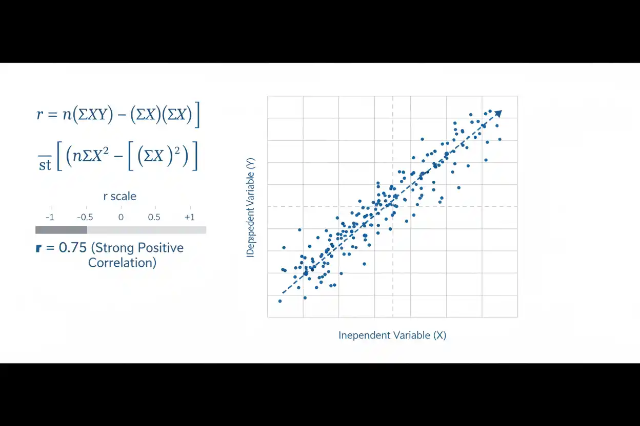
A correlation coefficient is a numerical measure that describes the strength and direction of association between two variables. The most familiar form, Pearson’s correlation coefficient, measures the strength of a linear relationship and takes values from −1 to +1. A positive correlation coefficient indicates that larger values of one variable tend to occur with larger values of the other, while a negative value indicates that larger values of one variable tend to occur with smaller values of the other. A value near zero indicates little linear association, although a strong nonlinear relationship can still exist. The magnitude of a correlation coefficient describes the strength of linear association, but its practical meaning depends on the subject area, data quality, range of observations, and study design. Correlation does not by itself establish causation, and a statistically significant correlation coefficient can still represent a weak relationship in a sufficiently large sample. Outliers can also alter Pearson’s correlation coefficient substantially, so the numerical result should be interpreted together with a scatter plot and the structure of the data.
The correlation coefficient is a central measure of association within core statistics and the broader Statistics & Probability framework. It is closely related mathematically to covariance, but standardizing by the variables’ standard deviations gives the correlation coefficient its familiar dimensionless scale from −1 to +1.
What Is a Correlation Coefficient?
A correlation coefficient summarizes the degree to which two variables vary together according to a specified form of association.
For Pearson’s correlation coefficient, the focus is linear association.
The population Pearson correlation coefficient is usually represented by:
ρ
The sample correlation coefficient is represented by:
r
The possible range is:
−1 ≤ r ≤ 1
A value of:
r = 1
represents a perfect positive linear relationship.
A value of:
r = −1
represents a perfect negative linear relationship.
A value of:
r = 0
indicates zero sample linear correlation.
However, zero correlation does not necessarily mean the variables are unrelated. They may have a strong curved or otherwise nonlinear relationship that Pearson’s correlation coefficient does not capture.
Correlation Coefficient Formula
For paired sample observations:
(x₁, y₁), (x₂, y₂), …, (xₙ, yₙ)
Pearson’s sample correlation coefficient can be calculated as:
r = Σ[(xᵢ − x̄)(yᵢ − ȳ)] / √[Σ(xᵢ − x̄)² Σ(yᵢ − ȳ)²]
where:
- xᵢ = individual observation of variable X
- yᵢ = corresponding observation of variable Y
- x̄ = sample mean of X
- ȳ = sample mean of Y
- n = number of paired observations
- r = sample Pearson correlation coefficient
The numerator measures how the two variables vary together.
The denominator scales that joint variation according to the variability of each variable.
This standardization is what constrains the correlation coefficient to the interval:
[−1, 1]
Correlation Coefficient Using Covariance
Pearson’s population correlation coefficient can also be written:
ρₓᵧ = Cov(X, Y)/(σₓσᵧ)
For sample data:
r = sₓᵧ/(sₓsᵧ)
where:
- sₓᵧ = sample covariance
- sₓ = sample standard deviation of X
- sᵧ = sample standard deviation of Y
This relationship explains the connection between a correlation coefficient and covariance.
Covariance indicates the direction of joint variation, but its magnitude depends on the units of the variables.
The correlation coefficient removes those units by dividing covariance by both standard deviations.
As a result, correlation can be compared across variables measured on very different scales.
Why Correlation Is Dimensionless
Suppose X is measured in kilograms and Y in centimeters.
Their covariance has units related to:
kilograms × centimeters
If either variable is converted to another positive linear unit, the numerical covariance changes.
Pearson’s correlation coefficient divides covariance by:
σₓσᵧ
which carries the same product of measurement units.
The units therefore cancel.
The correlation coefficient is consequently dimensionless.
For example, converting height from centimeters to meters does not change Pearson’s correlation coefficient, provided the transformation is positive and linear.
Interpreting the Sign of a Correlation Coefficient
The sign indicates the direction of the linear relationship.
Positive Correlation
If:
r > 0
larger X values tend to be associated with larger Y values.
For example:
r = 0.78
indicates a positive linear association.
This does not mean Y always increases whenever X increases. Individual observations can deviate substantially from the overall trend.
Negative Correlation
If:
r < 0
larger X values tend to be associated with smaller Y values.
For example:
r = −0.78
has the same magnitude as +0.78 but the opposite direction.
Zero Correlation
If:
r = 0
the sample has no linear correlation.
This should not be interpreted automatically as:
“There is no relationship.”
A nonlinear relationship can produce a correlation coefficient close to zero.
Interpreting the Magnitude
The absolute value:
|r|
describes the strength of the linear relationship.
Values closer to:
1
indicate observations that more closely follow a straight-line pattern.
Values closer to:
0
indicate weaker linear association.
A rough descriptive scale is sometimes presented as:
| |r| | Possible Description |
|—:|—|
| 0.00–0.19 | Very weak |
| 0.20–0.39 | Weak |
| 0.40–0.59 | Moderate |
| 0.60–0.79 | Strong |
| 0.80–1.00 | Very strong |
These labels should not be treated as universal statistical rules.
In one scientific field, r = 0.30 may be substantively important. In another context, even r = 0.80 may be considered insufficient for a predictive application.
The numerical correlation coefficient should therefore be interpreted in context rather than classified mechanically.
Correlation Coefficient Example
Consider the following paired observations:
| X | Y |
|---|---|
| 1 | 2 |
| 2 | 4 |
| 3 | 5 |
| 4 | 4 |
| 5 | 5 |
We will calculate Pearson’s correlation coefficient.
Step 1: Calculate the Means
For X:
x̄ = (1 + 2 + 3 + 4 + 5)/5
x̄ = 3
For Y:
ȳ = (2 + 4 + 5 + 4 + 5)/5
ȳ = 4
Step 2: Calculate Deviations From the Means
| X | Y | xᵢ − x̄ | yᵢ − ȳ | (xᵢ − x̄)(yᵢ − ȳ) |
|---|---|---|---|---|
| 1 | 2 | −2 | −2 | 4 |
| 2 | 4 | −1 | 0 | 0 |
| 3 | 5 | 0 | 1 | 0 |
| 4 | 4 | 1 | 0 | 0 |
| 5 | 5 | 2 | 1 | 2 |
Therefore:
Σ[(xᵢ − x̄)(yᵢ − ȳ)] = 6
Step 3: Calculate Squared Deviations
For X:
Σ(xᵢ − x̄)² = 4 + 1 + 0 + 1 + 4
= 10
For Y:
Σ(yᵢ − ȳ)² = 4 + 0 + 1 + 0 + 1
= 6
Step 4: Apply the Correlation Coefficient Formula
r = 6/√(10 × 6)
r = 6/√60
r ≈ 0.7746
Therefore:
r ≈ 0.775
The sample shows a fairly strong positive linear association.
As X increases, Y tends to increase as well, although the relationship is not perfectly linear.
What Does r = 1 Mean?
A correlation coefficient of:
r = 1
means all sample points lie exactly on a straight line with positive slope.
For example:
Y = 2X + 3
would produce:
r = 1
as long as X varies.
Every increase in X is associated with an exact linear increase in Y.
However, r = 1 does not require:
Y = X
The slope can be any positive value.
The defining condition is perfect positive linear association.
What Does r = −1 Mean?
A value of:
r = −1
means every point lies exactly on a straight line with negative slope.
For example:
Y = 10 − 2X
produces a perfect negative linear relationship.
As X increases, Y decreases in an exact linear pattern.
The strength is perfect because:
|r| = 1
and the negative sign specifies the direction.
What Does r = 0 Mean?
A correlation coefficient of zero means there is no linear association in the sample.
Consider a relationship such as:
Y = X²
with X values distributed symmetrically around zero.
Y clearly depends on X, yet Pearson’s correlation coefficient can be zero because positive and negative linear contributions cancel.
Therefore:
r ≈ 0
should be interpreted as weak or absent linear association rather than proof of statistical independence or complete absence of relationship.
A scatter plot is essential for detecting patterns that a single correlation coefficient may hide.
Correlation Coefficient and Scatter Plots
A correlation coefficient compresses a relationship into one number.
A scatter plot reveals its structure.
Two data sets can have similar correlation coefficients but very different shapes because of:
- outliers,
- clusters,
- nonlinear relationships,
- restricted ranges,
- subgroups,
- heteroscedasticity.
Before interpreting Pearson’s correlation coefficient, it is generally useful to inspect a scatter plot.
A coefficient such as:
r = 0.70
is much easier to understand when the observed points can also be examined visually.
Correlation Coefficient and Covariance
The sample covariance is:
sₓᵧ = Σ[(xᵢ − x̄)(yᵢ − ȳ)]/(n − 1)
For the example:
sₓᵧ = 6/(5 − 1)
sₓᵧ = 1.5
The sample standard deviations are:
sₓ = √[10/(5 − 1)]
sₓ = √2.5
sₓ ≈ 1.5811
and:
sᵧ = √[6/(5 − 1)]
sᵧ = √1.5
sᵧ ≈ 1.2247
Then:
r = 1.5/(1.5811 × 1.2247)
r ≈ 0.7746
This produces the same result as the direct correlation coefficient formula.
The difference is interpretive: covariance depends on measurement units, while correlation standardizes the relationship.
Sample Correlation vs Population Correlation
The population correlation coefficient is:
ρ
The sample correlation coefficient is:
r
A sample correlation coefficient is a statistic calculated from observed sample data.
The population correlation coefficient is a parameter describing the corresponding association in the population.
Therefore:
r
is commonly used as an estimate of:
ρ
Sampling variation means r will generally not equal ρ exactly.
Different random samples from the same population can produce different sample correlation coefficients.
This is why estimation and inference are necessary when conclusions about a population correlation are required.
Correlation Coefficient and Statistical Significance
A nonzero sample correlation coefficient does not automatically establish a nonzero population correlation.
A hypothesis test for Pearson correlation often evaluates:
H₀: ρ = 0
against an alternative such as:
H₁: ρ ≠ 0
Under the usual assumptions, the test statistic is:
t = r√[(n − 2)/(1 − r²)]
with:
df = n − 2
when testing zero population correlation.
The resulting statistic is compared with a t reference distribution.
The relevant critical values or p-value determine whether the sample provides sufficient evidence against H₀ at a chosen significance level.
Correlation Significance Example
Using:
r ≈ 0.7746
and:
n = 5
the test statistic is:
t = 0.7746√[(5 − 2)/(1 − 0.7746²)]
Since:
r² = 0.6
we have:
t = 0.7746√(3/0.4)
t = 0.7746√7.5
t ≈ 2.121
The degrees of freedom are:
df = 5 − 2
df = 3
Although r appears fairly strong, the sample is extremely small. A two-sided test at α = 0.05 would not reject H₀ because the required evidence is stronger with only three degrees of freedom.
This illustrates an important principle:
A large-looking correlation coefficient and statistical significance are not the same thing.
Sample size strongly affects inferential uncertainty.
Statistical Significance vs Strength of Correlation
The magnitude of r and its p-value answer different questions.
The correlation coefficient describes the observed strength and direction of linear association.
The p-value describes how incompatible the observed statistic is with a specified null model.
With a very large sample, a small correlation such as:
r = 0.08
may be statistically significant.
With a very small sample, a seemingly large correlation such as:
r = 0.70
may not be statistically significant.
Neither result should be interpreted using significance alone.
Effect magnitude, uncertainty, sample size, study design, and practical importance all matter.
Confidence Intervals for a Correlation Coefficient
A sample correlation coefficient can also be accompanied by a confidence interval for the population correlation ρ.
Because the sampling distribution of r is not generally symmetric, particularly when the population correlation is far from zero, confidence intervals are often constructed using Fisher’s z transformation.
The transformation is:
z = 0.5 ln[(1 + r)/(1 − r)]
Its approximate standard error is:
SE_z = 1/√(n − 3)
for suitable conditions.
A confidence interval is constructed on the transformed scale and then converted back to the correlation scale.
The general interpretation of such an interval follows the principles discussed for confidence intervals and the selected confidence level.
Correlation Coefficient and the Coefficient of Determination
For a simple linear relationship involving one predictor, squaring Pearson’s correlation coefficient gives:
r²
This is closely related to the coefficient of determination in simple linear regression.
For the example:
r ≈ 0.7746
so:
r² ≈ 0.60
In a simple linear regression with an intercept, this means approximately 60% of the sample variation in Y around its mean is accounted for by the fitted linear relationship with X.
However, it is important not to overgeneralize this interpretation.
The statement:
“60% of Y is caused by X”
would be incorrect.
The r² value describes linear explanatory fit in that model, not causal contribution.
Correlation Does Not Imply Causation
One of the most important limitations of a correlation coefficient is that association does not establish causal direction.
Suppose X and Y have:
r = 0.85
Several possibilities remain:
- X may influence Y.
- Y may influence X.
- A third variable may influence both.
- Selection effects may create the association.
- Measurement or sampling processes may contribute.
- The relationship may be partly or entirely noncausal.
The correlation coefficient itself cannot distinguish these explanations.
Causal inference requires study design, temporal information, assumptions about confounding, and substantive evidence beyond the magnitude of r.
Confounding and Correlation
A confounding variable can produce an apparent relationship between X and Y even when neither directly causes the other.
For example, two variables may both increase with age.
If age is not considered, the two variables may show a strong positive correlation.
The observed correlation coefficient then reflects at least partly their shared relationship with age.
This does not make the correlation mathematically incorrect. It means the interpretation must consider the broader system generating the data.
Correlation describes association in the observed data; it does not automatically explain its source.
Correlation Coefficient and Outliers
Pearson’s correlation coefficient can be highly sensitive to extreme observations.
A single point far from the main data cloud can:
- strengthen the apparent linear relationship,
- weaken an otherwise strong relationship,
- reverse the apparent direction,
- create a correlation where the main observations show little pattern.
Consider a sample where most points form a nearly circular cloud around the origin.
Adding one extreme point in the upper-right corner may create a substantial positive correlation coefficient.
This is another reason to examine the scatter plot rather than relying solely on r.
Outliers should be investigated rather than automatically removed.
Restricted Range
Restricting the range of one or both variables can reduce the observed correlation coefficient.
Suppose height and weight have a positive relationship across adults of many sizes.
If the sample contains only people within a very narrow height range, much of the variation needed to reveal the relationship has been removed.
The resulting correlation may be much smaller than in the broader population.
Therefore, a correlation coefficient depends partly on the range of data included in the analysis.
Comparisons of correlations across studies should consider differences in sampling and variable ranges.
Nonlinear Relationships
Pearson’s correlation coefficient specifically measures linear association.
Consider:
Y = X²
Across a symmetric range of X values, the relationship is perfectly deterministic but curved.
The Pearson correlation coefficient can be:
r ≈ 0
because the negative-X and positive-X portions of the curve contribute in opposing linear directions.
Therefore, a low correlation coefficient does not prove that X provides no information about Y.
It means there is little linear association according to Pearson’s measure.
Correlation Coefficient and Linearity
For Pearson’s correlation coefficient to summarize a relationship meaningfully, the pattern should be reasonably linear.
If the scatter plot bends strongly, r can understate or misrepresent the association.
For example, a curve that rises sharply and then levels off may have a moderate Pearson correlation coefficient even though Y changes systematically with X.
In such cases, nonlinear modeling or another measure of association may be more appropriate.
The correct measure should match the form of relationship being investigated.
Correlation Coefficient and Independence
If two random variables are statistically independent and have finite variances, their covariance is zero and therefore their Pearson correlation is zero.
Thus:
Independence ⇒ zero correlation
under the required moment conditions.
The reverse is not generally true:
Zero correlation ⇏ independence
Two variables can be dependent yet uncorrelated.
The relationship:
Y = X²
with suitably symmetric X provides a standard example.
This distinction is fundamental because correlation captures only a particular form of dependence.
Effect of Changing Units
Pearson’s correlation coefficient is unchanged by positive linear changes of measurement scale.
Suppose:
X* = a + bX
with:
b > 0
and:
Y* = c + dY
with:
d > 0
Then:
Corr(X*, Y*) = Corr(X, Y)
Adding constants changes the location of variables but not their correlation.
Multiplying by positive constants changes scale but not correlation.
If one variable is multiplied by a negative constant, the sign of the correlation reverses.
For example:
Corr(X, −Y) = −Corr(X, Y)
Correlation Is Symmetric
Pearson’s correlation coefficient has the property:
Corr(X, Y) = Corr(Y, X)
Therefore, the correlation between X and Y is identical to the correlation between Y and X.
This distinguishes correlation from prediction or regression, where specifying which variable is treated as the response can matter.
Correlation does not designate one variable as dependent and the other as independent.
It simply measures their linear association.
Correlation Coefficient With Constant Variables
Pearson’s correlation coefficient is undefined when either variable has zero variance.
Suppose every X observation equals:
X = 5
Then:
sₓ = 0
Since the correlation formula contains:
sₓsᵧ
in the denominator, division by zero would be required.
Therefore, a correlation coefficient cannot be calculated meaningfully when either variable is constant.
There must be variation in both variables.
Pearson vs Spearman Correlation
Pearson’s correlation coefficient measures linear association using the original numerical values.
Spearman’s rank correlation instead measures the strength of a monotonic relationship using ranks.
A relationship is monotonic when one variable generally moves in one direction as the other changes, even if the pattern is not linear.
Spearman correlation can therefore be useful when:
- the relationship is monotonic but nonlinear,
- ranks are more meaningful than raw distances,
- ordinal data are analyzed,
- extreme values make Pearson correlation unsuitable.
The two coefficients answer related but different questions.
A data set can have different Pearson and Spearman correlation values.
Pearson vs Kendall Correlation
Kendall’s tau is another rank-based measure of association.
It is based on concordant and discordant pairs rather than the raw numerical distances used by Pearson’s correlation coefficient.
Kendall’s tau can be particularly useful for ordinal data and smaller samples, depending on the inferential objective.
Pearson, Spearman, and Kendall coefficients should not be selected merely by comparing which one gives the largest number.
The choice should depend on measurement scale, relationship structure, assumptions, and the question being asked.
Assumptions for Pearson Correlation Inference
Calculating a descriptive Pearson correlation coefficient requires paired numerical data with variation in both variables.
Formal hypothesis tests and confidence intervals can require additional assumptions.
Important considerations include:
Independent Paired Observations
Each observation pair should represent an appropriate independent unit under the standard model.
Repeated observations from the same person or clustered data can require methods that account for dependence.
Linear Relationship
Pearson’s correlation coefficient is designed to quantify linear association.
A strong curved pattern can make r misleading.
Absence of Highly Influential Outliers
Extreme observations can dominate the coefficient.
Scatter plots and diagnostic analysis should therefore accompany the numerical result.
Distributional Assumptions for Classical Inference
Classical small-sample tests for Pearson correlation are commonly derived under a bivariate normal model.
Large-sample methods can be more robust in some situations, but they do not correct every problem involving dependence, selection bias, nonlinear structure, or extreme outliers.
Correlation Coefficient and Chi-Square
The chi-square method typically evaluates categorical frequency data.
Pearson’s correlation coefficient instead describes linear association between quantitative variables.
For example, if both X and Y are numerical measurements, a correlation coefficient may be suitable.
If both variables are categorical and observations are arranged in a contingency table, a chi-square test of independence may be more appropriate.
The fact that both procedures concern “relationships between variables” does not make them interchangeable.
The measurement scale and statistical question determine which method is appropriate.
Correlation Coefficient vs Covariance
Both covariance and correlation describe how two variables vary together.
Covariance is:
sₓᵧ = Σ[(xᵢ − x̄)(yᵢ − ȳ)]/(n − 1)
The correlation coefficient is:
r = sₓᵧ/(sₓsᵧ)
The main differences are:
| Property | Covariance | Correlation Coefficient |
|---|---|---|
| Direction | Yes | Yes |
| Standardized | No | Yes |
| Units | Product of variable units | Unitless |
| Fixed range | No | −1 to +1 |
| Strength easily comparable | Limited | Much easier |
Covariance is fundamental mathematically, while correlation is often easier to interpret across different measurement scales.
Correlation Coefficient vs Regression
Correlation measures the strength and direction of association.
Regression models a response variable as a function of one or more predictors.
In simple linear regression:
ŷ = a + bx
correlation and the regression slope are related, but they are not the same quantity.
The slope has units:
units of Y / units of X
while r is unitless.
The slope also changes if X or Y is rescaled, whereas Pearson’s correlation coefficient does not change under positive linear rescaling.
Regression additionally distinguishes between the predictor and response, while correlation is symmetric.
Correlation Coefficient and Exponential Relationships
An exponential regression model may be appropriate when the relationship between X and Y follows a curved pattern such as:
y = abˣ
A Pearson correlation coefficient on the original X and Y values may fail to summarize such a relationship effectively because it focuses on straight-line association.
In some settings, a suitable transformation can make the relationship approximately linear, after which correlation may help summarize the transformed variables.
However, transforming data should be justified by the model rather than performed solely to increase the correlation coefficient.
Correlation Coefficient and Sample Size
The numerical value of r does not mechanically increase or decrease with sample size.
However, sample size strongly influences the uncertainty surrounding r.
Suppose two samples both produce:
r = 0.30
If one has:
n = 20
and the other:
n = 2,000
the second estimate is generally much more precise under comparable sampling conditions.
A weak correlation can therefore be statistically significant in a large sample, while a stronger-looking correlation may remain uncertain in a small sample.
This is why reporting sample size and uncertainty is important.
Correlation Coefficient and Practical Significance
A statistically significant correlation coefficient is not automatically useful.
Suppose a study with hundreds of thousands of observations finds:
r = 0.04
The p-value may be extremely small because the estimate is precise.
Yet:
r² = 0.0016
so the simple linear association accounts for only a very small fraction of variation in the sample.
Whether that relationship matters depends on the application.
In some contexts, even small associations can be meaningful. In others, they may have negligible practical value.
Correlation Coefficient and Multiple Groups
A single overall correlation coefficient can sometimes conceal different relationships within subgroups.
For example, two groups may each show positive associations, while the pooled data show a negative association because the groups have different locations.
Conversely, an overall correlation may appear strong only because observations belong to distinct clusters.
This type of aggregation problem shows why subgroup structure should be considered before interpreting a single coefficient.
Statistical summaries can change when data are pooled across heterogeneous populations.
Correlation Coefficient and Missing Data
Missing observations can affect the correlation coefficient depending on how they are handled.
If only complete X-Y pairs are used, the analysis is based on the subset for which both variables are observed.
This can be reasonable when missingness is unrelated to the variables in a way that would distort the sample, but systematic missingness can introduce bias.
Different software may also use different missing-data rules, especially when calculating a full correlation matrix.
The reported coefficient should therefore be interpreted in light of the actual observations contributing to it.
Common Correlation Coefficient Mistakes
A major mistake is interpreting correlation as causation. A high correlation coefficient does not establish a causal mechanism.
Another is assuming that:
r = 0
means the variables are independent. Zero Pearson correlation rules out linear association but not every form of dependence.
A third error is interpreting the magnitude without examining a scatter plot. Outliers and nonlinear patterns can make the coefficient misleading.
It is also incorrect to compare the raw magnitude of covariance with a correlation coefficient because the measures use different scales.
Another common mistake is treating statistical significance as evidence of a strong association. With a large sample, a very small r can be statistically significant.
Analysts should also avoid mechanically labeling every correlation above a fixed threshold as “strong” regardless of context.
Finally, calculating Pearson correlation for a variable with zero variance is impossible because the denominator becomes zero.
How to Calculate a Correlation Coefficient Step by Step
A reliable manual calculation follows this sequence.
Step 1: Arrange the Data as Pairs
Every X value must correspond to the correct Y value:
(x₁, y₁), (x₂, y₂), …, (xₙ, yₙ)
Step 2: Calculate the Means
x̄ = Σxᵢ/n
ȳ = Σyᵢ/n
Step 3: Calculate Deviations
For each pair:
xᵢ − x̄
and:
yᵢ − ȳ
Step 4: Multiply Corresponding Deviations
(xᵢ − x̄)(yᵢ − ȳ)
Then sum:
Σ[(xᵢ − x̄)(yᵢ − ȳ)]
Step 5: Calculate Squared Deviations
Find:
Σ(xᵢ − x̄)²
and:
Σ(yᵢ − ȳ)²
Step 6: Calculate the Denominator
√[Σ(xᵢ − x̄)² Σ(yᵢ − ȳ)²]
Step 7: Divide
r = numerator/denominator
Step 8: Check the Range
The result must satisfy:
−1 ≤ r ≤ 1
A result outside that range indicates an arithmetic or implementation error.
Step 9: Interpret Direction and Strength
Use the sign for direction and the magnitude for linear strength.
Step 10: Examine the Data Structure
Check a scatter plot, outliers, nonlinear patterns, subgroup structure, and study design before drawing substantive conclusions.
How to Report a Correlation Coefficient
A useful report includes:
- the variables being correlated,
- the coefficient,
- sample size,
- uncertainty or test result when inferential claims are made,
- substantive interpretation.
For example:
Pearson’s r = 0.775, n = 5
If a hypothesis test is included, the result can be reported with the test statistic, degrees of freedom, and p-value.
The substantive statement should describe the association rather than imply unsupported causation.
For example:
The sample showed a positive linear association between X and Y.
is appropriate.
A statement such as:
X caused Y because r was positive
is not justified by the correlation coefficient alone.
Frequently Asked Questions About the Correlation Coefficient
What is a correlation coefficient?
A correlation coefficient is a numerical measure of the strength and direction of association between variables. Pearson’s correlation coefficient specifically measures linear association between two quantitative variables.
What is the formula for Pearson’s correlation coefficient?
The sample formula is:
r = Σ[(xᵢ − x̄)(yᵢ − ȳ)] / √[Σ(xᵢ − x̄)² Σ(yᵢ − ȳ)²]
What is the range of a correlation coefficient?
Pearson’s correlation coefficient always satisfies:
−1 ≤ r ≤ 1
provided it is defined.
What does a positive correlation coefficient mean?
A positive value means larger values of one variable tend to be associated with larger values of the other in a linear sense.
What does a negative correlation coefficient mean?
A negative value means larger values of one variable tend to be associated with smaller values of the other.
What does a correlation coefficient of 1 mean?
r = 1
indicates a perfect positive linear relationship.
What does a correlation coefficient of −1 mean?
r = −1
indicates a perfect negative linear relationship.
What does r = 0 mean?
It means the sample has zero Pearson linear correlation. It does not necessarily mean the variables are independent or unrelated.
Is r = 0.8 always a strong correlation?
It represents a strong linear association under many informal conventions, but practical interpretation depends on the field, data structure, sampling process, and purpose of the analysis.
Does correlation prove causation?
No. A correlation coefficient measures association. Causal interpretation requires additional design and substantive assumptions.
What is the difference between correlation and covariance?
Covariance measures joint variation in the original measurement units. Correlation standardizes covariance by the standard deviations of both variables, making the result unitless and constrained between −1 and +1.
What is the difference between Pearson and Spearman correlation?
Pearson correlation measures linear association using the numerical values themselves. Spearman correlation uses ranks and measures monotonic association.
Can a nonlinear relationship have zero correlation?
Yes. A strong nonlinear relationship can have a Pearson correlation coefficient of zero or close to zero.
Can an outlier affect the correlation coefficient?
Yes. Pearson’s correlation coefficient can be highly sensitive to influential observations, which can strengthen, weaken, or even reverse the apparent association.
Does sample size affect the correlation coefficient?
Sample size does not directly determine the numerical value of r, but it strongly affects the uncertainty and statistical significance associated with the estimate.
How do you test whether a correlation coefficient is statistically significant?
For testing:
H₀: ρ = 0
a common Pearson correlation test uses:
t = r√[(n − 2)/(1 − r²)]
with:
df = n − 2
under the appropriate assumptions.
Is a statistically significant correlation necessarily strong?
No. A small correlation coefficient can be statistically significant in a sufficiently large sample.
What is r²?
In simple linear regression with an intercept, r² is the coefficient of determination and represents the proportion of sample variation in the response accounted for by the fitted linear relationship.
Is correlation affected by measurement units?
Pearson’s correlation coefficient is unchanged by positive linear changes of scale such as converting centimeters to meters.
What happens if one variable is constant?
Pearson’s correlation coefficient is undefined because the constant variable has zero standard deviation, making the denominator of the formula zero.
Is correlation symmetric?
Yes:
Corr(X, Y) = Corr(Y, X)
Switching the order of the variables does not change Pearson’s correlation coefficient.




