


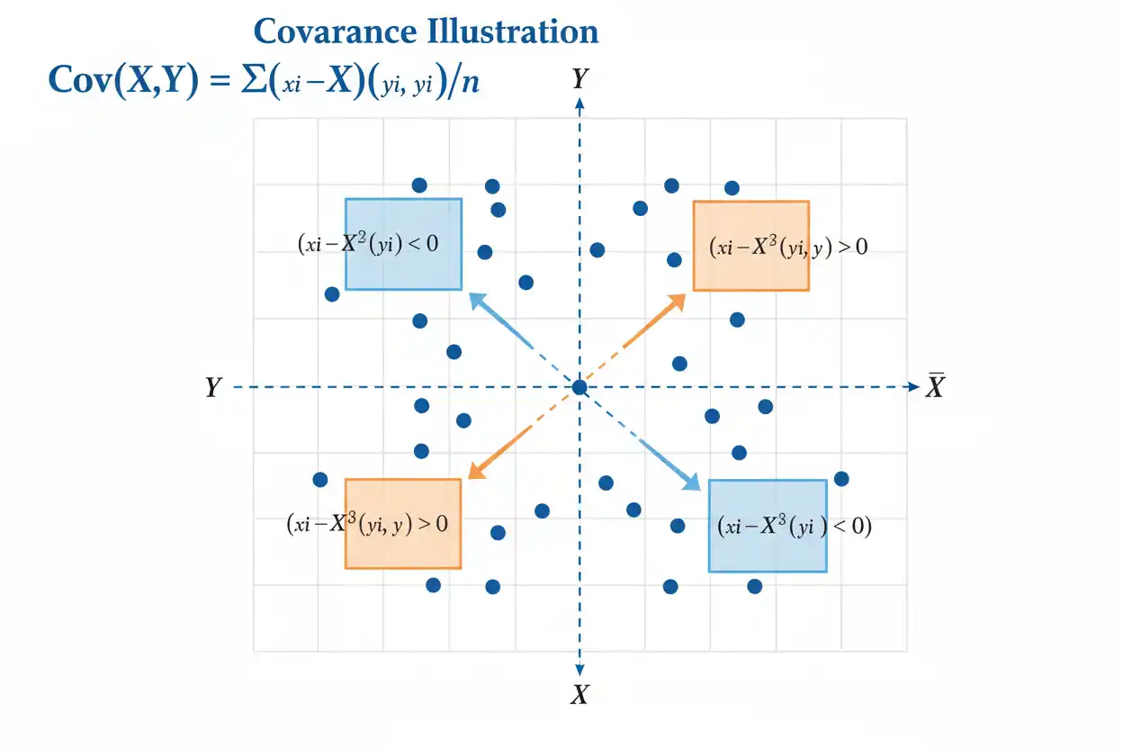
Covariance measures how two quantitative variables vary together. A positive covariance indicates that observations above the mean of one variable tend to occur with observations above the mean of the other, while values below their means also tend to occur together. A negative covariance indicates the opposite pattern: above-average values of one variable tend to accompany below-average values of the other. A covariance near zero indicates little average linear co-movement, but it does not prove that the variables are independent or unrelated. Unlike a correlation coefficient, covariance is not standardized, so its numerical magnitude depends on the units and scales of the variables. Population covariance and sample covariance also use different denominators, with N used for a complete population and n − 1 commonly used when sample data estimate a population covariance. Covariance is foundational in correlation, regression, portfolio analysis, multivariate statistics, and covariance matrices, but its raw magnitude must always be interpreted in context.
Within core statistics, covariance provides one of the basic mathematical measures of joint variability. The broader Statistics & Probability framework builds on this idea through estimation, distributions, hypothesis testing, and standardized measures such as the correlation coefficient.
What Is Covariance?
Covariance describes whether two variables tend to deviate from their respective means in the same direction or in opposite directions.
Suppose X and Y are measured for the same observational units.
For each observation, compare:
xᵢ − x̄
with:
yᵢ − ȳ
If both deviations are positive, their product is positive.
If both deviations are negative, their product is also positive.
If one deviation is positive and the other negative, their product is negative.
Covariance averages these paired deviation products.
The sign therefore reveals the general direction of linear co-movement:
Covariance > 0 → variables tend to move in the same direction.
Covariance < 0 → variables tend to move in opposite directions.
Covariance ≈ 0 → little average linear co-movement.
However, the last statement must be interpreted carefully. Zero covariance does not generally imply independence.
Population Covariance Formula
For two population variables X and Y, covariance is:
Cov(X, Y) = E[(X − μₓ)(Y − μᵧ)]
where:
- μₓ = population mean of X
- μᵧ = population mean of Y
- E = expected value
For a finite population containing N paired observations, the corresponding formula is:
σₓᵧ = Σ(xᵢ − μₓ)(yᵢ − μᵧ)/N
where:
- xᵢ = ith population value of X
- yᵢ = corresponding population value of Y
- N = number of population pairs
- σₓᵧ = population covariance
This formula averages the products of the deviations from the two population means.
Sample Covariance Formula
When a sample is used to estimate population covariance, the usual sample covariance is:
sₓᵧ = Σ(xᵢ − x̄)(yᵢ − ȳ)/(n − 1)
where:
- x̄ = sample mean of X
- ȳ = sample mean of Y
- n = number of paired observations
- sₓᵧ = sample covariance
The denominator is:
n − 1
rather than:
n
because the deviations are calculated around sample means estimated from the same data.
The n − 1 denominator gives the conventional unbiased estimator of population covariance under independent sampling with finite second moments.
This population-versus-sample distinction is analogous to the distinction between population and sample variance.
Why Sample Covariance Uses n − 1
When x̄ and ȳ are calculated from the sample, the deviations are constrained by:
Σ(xᵢ − x̄) = 0
and:
Σ(yᵢ − ȳ) = 0
The sample means have already been estimated from the observations, which reduces the effective degrees of freedom.
Using:
n − 1
corrects the systematic downward bias that would otherwise occur if the centered cross-products were simply divided by n when estimating population covariance.
Thus:
Population covariance → divide by N
Sample covariance estimator → divide by n − 1
The choice depends on whether the data represent the full population of interest or a sample being used for inference.
Covariance Example
Consider five paired observations:
| X | Y |
|---|---|
| 1 | 2 |
| 2 | 1 |
| 3 | 4 |
| 4 | 3 |
| 5 | 5 |
We will calculate the sample covariance.
Step 1: Calculate the Means
For X:
x̄ = (1 + 2 + 3 + 4 + 5)/5
x̄ = 3
For Y:
ȳ = (2 + 1 + 4 + 3 + 5)/5
ȳ = 3
Step 2: Calculate Deviations
| X | Y | xᵢ − x̄ | yᵢ − ȳ |
|---|---|---|---|
| 1 | 2 | −2 | −1 |
| 2 | 1 | −1 | −2 |
| 3 | 4 | 0 | 1 |
| 4 | 3 | 1 | 0 |
| 5 | 5 | 2 | 2 |
Step 3: Multiply Corresponding Deviations
| xᵢ − x̄ | yᵢ − ȳ | Product |
|---|---|---|
| −2 | −1 | 2 |
| −1 | −2 | 2 |
| 0 | 1 | 0 |
| 1 | 0 | 0 |
| 2 | 2 | 4 |
The sum of the cross-products is:
Σ(xᵢ − x̄)(yᵢ − ȳ) = 2 + 2 + 0 + 0 + 4
= 8
Step 4: Divide by n − 1
Because this is sample covariance:
n = 5
so:
n − 1 = 4
Therefore:
sₓᵧ = 8/4
sₓᵧ = 2
The sample covariance is:
2
Because the result is positive, the two variables tend to deviate from their means in the same direction.
How to Interpret Positive Covariance
A positive covariance means that above-average values of X tend to occur with above-average values of Y, while below-average X values tend to occur with below-average Y values.
In the example, the pair:
X = 1, Y = 2
lies below both means:
x̄ = 3
ȳ = 3
Its covariance contribution is therefore positive:
(1 − 3)(2 − 3) = (−2)(−1) = 2
Likewise:
X = 5, Y = 5
lies above both means and contributes:
(5 − 3)(5 − 3) = 4
Positive covariance does not mean that every individual pair follows the same direction. It describes the net average of all paired deviation products.
How to Interpret Negative Covariance
Negative covariance occurs when the variables tend to deviate from their means in opposite directions.
Suppose larger X values tend to occur with smaller Y values.
Then many observations may have:
xᵢ − x̄ > 0
while:
yᵢ − ȳ < 0
giving:
(xᵢ − x̄)(yᵢ − ȳ) < 0
Likewise, observations below the X mean may occur above the Y mean, producing additional negative products.
When those negative cross-products dominate the sum:
Cov(X, Y) < 0
The covariance indicates negative linear co-movement.
What Does Zero Covariance Mean?
If:
Cov(X, Y) = 0
the average product of the centered variables is zero.
This means the variables are uncorrelated in the covariance sense.
It does not generally imply:
X and Y are independent.
A nonlinear relationship can produce zero covariance even when one variable depends completely on the other.
For example, suppose:
Y = X²
and X has a distribution symmetric around zero.
Large positive and negative X values both correspond to large Y values. The relationship is strong and deterministic, but the positive and negative cross-products can cancel, producing:
Cov(X, Y) = 0
Therefore:
Independence can imply zero covariance under suitable finite-moment conditions.
but:
Zero covariance does not generally imply independence.
Covariance and Independence
If X and Y are independent and have finite expected values, then:
E(XY) = E(X)E(Y)
Using an equivalent covariance formula:
Cov(X, Y) = E(XY) − E(X)E(Y)
we obtain:
Cov(X, Y) = 0
Therefore, under suitable moment conditions:
Independence ⇒ zero covariance
The reverse implication fails in general.
An important special case occurs with jointly normal variables. Under a joint normal distribution, zero covariance does imply independence.
That is a special property of the multivariate normal model and should not be generalized to arbitrary distributions.
Alternative Covariance Formula
Starting from:
Cov(X, Y) = E[(X − μₓ)(Y − μᵧ)]
expand the product:
(X − μₓ)(Y − μᵧ)
= XY − Xμᵧ − μₓY + μₓμᵧ
Taking expectations gives:
Cov(X, Y) = E(XY) − μₓμᵧ
because:
E(X) = μₓ
and:
E(Y) = μᵧ
Therefore:
Cov(X, Y) = E(XY) − E(X)E(Y)
This form is often useful in theoretical probability calculations.
For a finite population:
Cov(X, Y) = Σxᵢyᵢ/N − μₓμᵧ
when all terms refer consistently to the population.
Computational Formula for Sample Covariance
Sample covariance can also be written in an algebraically equivalent form:
sₓᵧ = [Σxᵢyᵢ − n x̄ȳ]/(n − 1)
Because:
n x̄ȳ = (Σxᵢ)(Σyᵢ)/n
another equivalent expression is:
sₓᵧ = [Σxᵢyᵢ − (Σxᵢ)(Σyᵢ)/n]/(n − 1)
These formulas can be convenient for manual calculation.
However, the centered formula:
sₓᵧ = Σ(xᵢ − x̄)(yᵢ − ȳ)/(n − 1)
usually makes the statistical meaning of covariance clearer.
With numerical computation involving very large values and small deviations, centered algorithms can also offer better numerical stability than naive computational formulas.
Covariance vs Correlation Coefficient
Covariance and the correlation coefficient both describe joint variation, but correlation standardizes covariance.
For sample data:
r = sₓᵧ/(sₓsᵧ)
where:
- sₓᵧ = sample covariance
- sₓ = sample standard deviation of X
- sᵧ = sample standard deviation of Y
Covariance has no fixed numerical range.
Correlation always satisfies:
−1 ≤ r ≤ 1
provided both variables have positive finite standard deviations.
This standardization makes correlation easier to compare across different variables and measurement scales.
Correlation From the Covariance Example
For the earlier data:
sₓᵧ = 2
The squared deviations of X sum to:
10
so:
sₓ² = 10/4 = 2.5
and:
sₓ = √2.5
sₓ ≈ 1.5811
The squared deviations of Y also sum to:
10
so:
sᵧ² = 2.5
and:
sᵧ ≈ 1.5811
Therefore:
r = 2/(1.5811 × 1.5811)
r = 2/2.5
r = 0.8
The sample covariance is:
2
while the sample correlation is:
0.8
The positive sign agrees in both measures, but the correlation is standardized and therefore immediately interpretable on the −1 to +1 scale.
Why Covariance Magnitude Is Difficult to Interpret
Suppose one study reports:
Cov(X, Y) = 12
and another reports:
Cov(A, B) = 400
It would be incorrect to conclude automatically that A and B have a stronger relationship.
The larger value may simply result from larger measurement units or more variable variables.
For example, converting a variable from meters to centimeters multiplies its numerical values by 100.
That conversion also multiplies its covariance with another variable by 100, even though the underlying relationship has not changed.
Raw covariance therefore communicates direction clearly but not standardized strength.
Units of Covariance
Covariance has units equal to the product of the units of the two variables.
Suppose:
X = height in centimeters
and:
Y = weight in kilograms
Then covariance has units:
centimeter·kilogram
If X is instead measured in meters, the numerical covariance changes because the scale of X changes.
This unit dependence is one major reason standardized correlation is often preferred when the goal is to describe relationship strength.
However, covariance remains essential in statistical formulas because retaining scale can be mathematically useful.
Effect of Adding a Constant
Adding a constant to either variable does not change covariance.
For constants a and b:
Cov(X + a, Y + b) = Cov(X, Y)
The reason is that adding a constant shifts the mean by the same amount.
For example:
(X + a) − E(X + a)
simplifies to:
X − E(X)
The centered deviations are unchanged.
Therefore, covariance is unaffected by changes in origin.
Converting Celsius to another scale that differs only by an additive constant would not change covariance, although a scale multiplication would.
Effect of Multiplying by a Constant
For constants a and b:
Cov(aX, bY) = ab Cov(X, Y)
Therefore, multiplying one variable by 10 multiplies the covariance by 10.
Multiplying both variables by 10 multiplies the covariance by:
10 × 10 = 100
If one multiplier is negative, the covariance sign changes.
For example:
Cov(−X, Y) = −Cov(X, Y)
This scaling property explains why the absolute magnitude of covariance cannot be interpreted without knowing the measurement scales.
Covariance of a Variable With Itself
A fundamental identity is:
Cov(X, X) = Var(X)
Starting from the definition:
Cov(X, X) = E[(X − μₓ)(X − μₓ)]
which becomes:
E[(X − μₓ)²]
That is exactly the population variance:
Var(X)
For sample data:
sₓₓ = sₓ²
Thus, variance can be viewed as a special case of covariance in which the two variables are the same.
This relationship is central to covariance matrices.
Covariance Is Symmetric
Covariance has the symmetry property:
Cov(X, Y) = Cov(Y, X)
This follows because multiplication is commutative:
(X − μₓ)(Y − μᵧ)
equals:
(Y − μᵧ)(X − μₓ)
Therefore, swapping the order of the variables does not change covariance.
This property also explains why covariance matrices are symmetric across their main diagonal.
Covariance With a Constant
If c is a constant:
Cov(X, c) = 0
A constant has no variability.
Its deviation from its own mean is always:
c − c = 0
Therefore, every centered cross-product is zero.
Likewise:
Cov(c, Y) = 0
This reinforces the idea that covariance measures joint variability. If one quantity does not vary, there can be no co-variation to measure.
Covariance of Sums
Covariance obeys useful algebraic rules.
For random variables X, Y, and Z:
Cov(X + Y, Z) = Cov(X, Z) + Cov(Y, Z)
More generally:
Cov(aX + bY, Z) = aCov(X, Z) + bCov(Y, Z)
These linearity properties make covariance particularly important when analyzing sums of random variables.
For example, the variance of a sum satisfies:
Var(X + Y) = Var(X) + Var(Y) + 2Cov(X, Y)
This formula shows directly why dependence between variables affects the variability of their sum.
Variance of a Sum
Because:
Var(X + Y) = Cov(X + Y, X + Y)
expand using covariance linearity:
Var(X + Y) = Var(X) + Var(Y) + 2Cov(X, Y)
If X and Y are uncorrelated:
Cov(X, Y) = 0
then:
Var(X + Y) = Var(X) + Var(Y)
If covariance is positive, the variance of the sum is larger than the sum of the separate variances.
If covariance is negative, the combined variance is reduced.
This property has major applications in multivariate modeling and risk aggregation.
Variance of a Difference
Similarly:
Var(X − Y) = Var(X) + Var(Y) − 2Cov(X, Y)
A positive covariance reduces the variance of the difference because the variables tend to move together.
A negative covariance increases the variance of the difference because opposite movements make the difference more variable.
These identities demonstrate why covariance is more than a descriptive association measure. It directly determines how uncertainties combine.
Covariance Matrix
When more than two variables are analyzed, their pairwise covariances can be organized into a covariance matrix.
For variables:
X₁, X₂, …, Xₚ
the covariance matrix Σ has the general form:
Σ =
[Var(X₁) Cov(X₁,X₂) … Cov(X₁,Xₚ)]
[Cov(X₂,X₁) Var(X₂) … Cov(X₂,Xₚ)]
[⋮ ⋮ ⋱ ⋮]
[Cov(Xₚ,X₁) Cov(Xₚ,X₂) … Var(Xₚ)]
The diagonal contains variances:
Cov(Xᵢ, Xᵢ) = Var(Xᵢ)
The off-diagonal elements contain pairwise covariances.
Because:
Cov(Xᵢ, Xⱼ) = Cov(Xⱼ, Xᵢ)
the matrix is symmetric.
Covariance matrices are fundamental in multivariate statistics, regression, principal-component methods, portfolio models, and many probability distributions.
Sample Covariance Matrix
Suppose three variables X, Y, and Z are observed.
Their sample covariance matrix can be represented as:
S =
[sₓ² sₓᵧ sₓz]
[sₓᵧ sᵧ² sᵧz]
[sₓz sᵧz sz²]
The diagonal entries describe the variability of each variable individually.
The off-diagonal values describe pairwise co-movement.
If:
sₓᵧ > 0
X and Y tend to move together.
If:
sₓz < 0
X and Z tend to move in opposite directions.
The full matrix summarizes the linear variance-covariance structure of the multivariate sample.
Positive Semidefinite Property
A valid covariance matrix has an important mathematical property: it is positive semidefinite.
For any vector a:
aᵀΣa ≥ 0
This follows because:
aᵀΣa
is the variance of a linear combination of the variables.
Variance cannot be negative.
This constraint matters when constructing or estimating covariance matrices because an arbitrary symmetric table of numbers is not necessarily a valid covariance matrix.
Covariance and Linear Regression
Covariance is closely related to the slope in simple linear regression.
For a regression model of Y on X, the ordinary least-squares slope can be written:
b₁ = Cov(X, Y)/Var(X)
using the corresponding sample or population quantities consistently.
For sample data:
b₁ = sₓᵧ/sₓ²
This formula shows that regression slope depends on joint variation between X and Y relative to the variation in X.
The covariance contributes direction and co-movement, while dividing by Var(X) converts that relationship into the units of a regression slope.
The wider regression framework also covers relationships that should not be reduced to covariance alone, including curved structures such as exponential regression.
Covariance and Exponential Relationships
Covariance is primarily a measure of linear co-movement.
If two variables follow a strong nonlinear relationship, their raw covariance can fail to summarize that structure adequately.
For example, an exponential relationship may have the form:
y = abˣ
Such a pattern can display positive covariance, but a single covariance value does not describe the shape, rate of growth, or predictive form of the relationship.
In settings where the relationship itself is exponential, an exponential regression model addresses the functional form more directly.
Covariance can still contribute to transformed or linearized calculations, but it should not replace an appropriate model of the relationship.
Covariance and Confidence Intervals
A sample covariance is an estimate of an unknown population covariance.
Like other sample statistics, it is subject to sampling variability.
A point estimate such as:
sₓᵧ = 2
does not reveal how much uncertainty surrounds the corresponding population covariance.
Inferential procedures can be used to quantify uncertainty, although confidence intervals for covariance can require distributional assumptions, transformations, asymptotic approximations, or resampling methods depending on the setting.
The general interpretation principles for confidence intervals still apply: an interval procedure should be understood through its long-run coverage properties rather than as a posterior probability statement about a fixed parameter.
The selected confidence level determines the nominal coverage target.
Covariance and Critical Values
When statistical inference about covariance or related parameters relies on a reference distribution, the relevant cutoff depends on the inferential method.
A critical value is determined by factors such as:
- reference distribution,
- tail structure,
- significance level,
- confidence level,
- degrees of freedom where relevant.
There is no universal covariance critical value.
The descriptive sample covariance itself does not require a critical value. Critical values become relevant when performing formal tests or constructing particular inferential procedures.
Covariance and Correlation Inference
Because population correlation satisfies:
ρ = Cov(X, Y)/(σₓσᵧ)
testing whether:
ρ = 0
is closely related to assessing whether the population covariance is zero when both population standard deviations are positive.
However, correlation is often the more interpretable target because it is standardized.
For example:
Cov(X, Y) = 20
cannot be evaluated as “large” or “small” without knowing the measurement scales.
A correlation of:
r = 0.80
immediately communicates strong positive linear association on a standardized scale, although its substantive importance still depends on context.
Covariance and Statistical Significance
The sign or size of a sample covariance does not by itself establish statistical significance.
A sample covariance can differ from zero simply because of sampling variation.
Formal inference requires a null hypothesis, sampling assumptions, and an appropriate test statistic or interval procedure.
For example, if the inferential target is linear association, analysts frequently test a population correlation rather than raw covariance because correlation has a standardized interpretation.
Regardless of the parameter, statistical significance should not be confused with practical importance.
A precisely estimated but substantively tiny relationship may be statistically significant in a large sample.
Covariance Does Not Prove Causation
Positive covariance does not mean that increases in X cause increases in Y.
Negative covariance does not mean that X causes Y to decrease.
Several explanations can generate covariance:
- X may influence Y.
- Y may influence X.
- another variable may influence both.
- selection effects may create the observed relationship.
- measurement structure may contribute.
- the association may be coincidental within the sample.
Covariance describes joint variability.
Causation requires additional assumptions and evidence concerning the process that generated the data.
Effect of Outliers on Covariance
Covariance is sensitive to extreme observations.
The formula contains products of deviations:
(xᵢ − x̄)(yᵢ − ȳ)
An observation far from both means can therefore contribute a very large positive or negative value.
An extreme point in the upper-right or lower-left portion of a scatter plot can strongly increase covariance.
An extreme point in the upper-left or lower-right can strongly decrease it.
Outliers should be investigated rather than automatically removed. They may reflect errors, unusual but valid observations, or evidence that the assumed model does not describe the data well.
Covariance and Centering
Covariance is based on deviations from the means rather than raw products alone.
This is crucial.
If we simply calculated:
average of xᵢyᵢ
the result would depend strongly on the absolute locations of X and Y.
Centering removes that location effect:
X − E(X)
Y − E(Y)
and focuses the calculation on joint deviations.
This is also why adding constants to variables leaves covariance unchanged.
The measure captures co-variation around each variable’s center.
Covariance and Standardization
Suppose X and Y are converted to z-scores:
Zₓ = (X − μₓ)/σₓ
Zᵧ = (Y − μᵧ)/σᵧ
Then:
Cov(Zₓ, Zᵧ) = Corr(X, Y)
Thus, correlation can be interpreted as the covariance of standardized variables.
Once both variables have:
mean = 0
and:
standard deviation = 1
their covariance becomes unitless and is constrained to:
−1 ≤ covariance ≤ 1
in that standardized setting.
This relationship provides a direct mathematical bridge between covariance and correlation.
Covariance and Binary Variables
Covariance is not limited to continuously measured variables.
A binary variable can be coded as:
1 = event occurs
0 = event does not occur
and covariance can then be calculated between binary indicators or between a binary variable and a quantitative variable.
However, interpretation depends on the coding scheme.
Changing the coding can change the scale or sign of covariance.
Therefore, the numerical value should always be interpreted together with the variable definitions.
For purely categorical contingency-table questions, methods such as chi-square may address the inferential objective more directly than raw covariance.
Covariance and Probability
For random variables X and Y:
Cov(X, Y) = E(XY) − E(X)E(Y)
This formula shows that covariance is fundamentally a probability concept based on expectations.
If:
E(XY) > E(X)E(Y)
covariance is positive.
If:
E(XY) < E(X)E(Y)
covariance is negative.
If:
E(XY) = E(X)E(Y)
covariance is zero.
Independence ensures the equality:
E(XY) = E(X)E(Y)
when the expectations exist, which explains why independent variables have zero covariance.
Covariance and Random Sums
Covariance becomes especially useful when calculating the variance of linear combinations.
Let:
W = aX + bY
Then:
Var(W) = a²Var(X) + b²Var(Y) + 2abCov(X, Y)
This formula shows explicitly how covariance affects combined uncertainty.
If covariance is positive and:
ab > 0
the covariance term increases Var(W).
If covariance is negative, it can reduce Var(W).
With many variables, the same principle extends naturally through a covariance matrix.
Why Covariance Matters in Multivariate Data
When analyzing one variable, variance describes its spread.
When analyzing many variables simultaneously, individual variances are not enough.
Analysts also need to know how the variables move together.
Two data sets can have exactly the same variance for every individual variable but very different joint structures because their covariances differ.
Covariance therefore provides information unavailable from separate univariate summaries.
This joint structure is fundamental to multivariate probability and statistics.
Common Covariance Mistakes
A common mistake is interpreting the magnitude of covariance as though it were standardized. A covariance of 100 is not automatically stronger than a covariance of 5 because the values may use different units and scales.
Another mistake is confusing population and sample formulas. Population covariance divides by N, while the conventional unbiased sample estimator divides by n − 1.
A third mistake is interpreting zero covariance as independence. Zero covariance only indicates the absence of linear co-movement in the covariance sense unless stronger distributional assumptions are present.
It is also incorrect to treat positive covariance as evidence of causation.
Another common error is calculating covariance from unpaired observations. Each xᵢ must correspond to the correct yᵢ for the same observational unit.
Outliers can also dominate covariance, so relying on the numerical value without inspecting the data can be misleading.
Finally, covariance should not be compared across differently scaled data sets without recognizing that changes in units alter the numerical result.
How to Calculate Sample Covariance Step by Step
A reliable manual procedure is straightforward.
Step 1: Confirm the Data Are Paired
Arrange observations as:
(x₁, y₁), (x₂, y₂), …, (xₙ, yₙ)
Each X value must correspond to the correct Y value.
Step 2: Calculate Both Sample Means
x̄ = Σxᵢ/n
ȳ = Σyᵢ/n
Step 3: Calculate Deviations
For each observation:
xᵢ − x̄
and:
yᵢ − ȳ
Step 4: Multiply the Paired Deviations
(xᵢ − x̄)(yᵢ − ȳ)
Step 5: Add All Cross-Products
Σ(xᵢ − x̄)(yᵢ − ȳ)
Step 6: Divide by n − 1
For sample covariance:
sₓᵧ = Σ(xᵢ − x̄)(yᵢ − ȳ)/(n − 1)
Step 7: Interpret the Sign
Positive → same-direction co-movement
Negative → opposite-direction co-movement
Near zero → little linear co-movement
Step 8: Consider Scale and Data Structure
Do not interpret magnitude without examining units, variability, outliers, scatter plots, and the purpose of the analysis.
How to Report Covariance
A useful covariance statement identifies the variables and units.
For example:
The sample covariance between X and Y was sₓᵧ = 2.
If the units are meaningful, they should also be stated.
A stronger interpretation might say:
The positive sample covariance indicates that observations above the mean of X tended to occur with observations above the mean of Y, and observations below their respective means also tended to occur together.
Avoid statements such as:
“A covariance of 2 means the relationship is strong.”
Raw covariance does not have a universal strength scale.
If standardized strength is needed, the correlation coefficient is usually more interpretable.
Frequently Asked Questions About Covariance
What is covariance?
Covariance measures how two quantitative variables vary together around their respective means.
What is the sample covariance formula?
The usual sample covariance is:
sₓᵧ = Σ(xᵢ − x̄)(yᵢ − ȳ)/(n − 1)
What is the population covariance formula?
For a finite population:
σₓᵧ = Σ(xᵢ − μₓ)(yᵢ − μᵧ)/N
More generally:
Cov(X, Y) = E[(X − μₓ)(Y − μᵧ)]
Why does sample covariance use n − 1?
The sample means are estimated from the same observations, reducing the effective degrees of freedom. Dividing by n − 1 gives the conventional unbiased estimator of population covariance.
What does positive covariance mean?
Positive covariance means the variables tend to deviate from their means in the same direction.
What does negative covariance mean?
Negative covariance means above-average values of one variable tend to occur with below-average values of the other, and vice versa.
What does zero covariance mean?
Zero covariance indicates no average linear co-movement. It does not generally prove that the variables are independent.
Does independence imply zero covariance?
Yes, when the relevant expectations and variances exist:
Independence ⇒ Cov(X, Y) = 0
The reverse is not generally true.
What is the difference between covariance and correlation?
Covariance measures joint variation in the original measurement scale. Correlation standardizes covariance by the standard deviations of both variables and is constrained between −1 and +1.
Can covariance be greater than 1?
Yes. Unlike correlation, covariance has no fixed −1 to +1 range. Its magnitude depends on the measurement scales of the variables.
Can covariance be less than −1?
Yes. Negative covariance can have any magnitude permitted by the variables’ scales and variability.
Can covariance be negative?
Yes. A negative result indicates opposite-direction linear co-movement.
Can covariance be zero even when variables are related?
Yes. Strong nonlinear dependence can produce zero covariance.
Is covariance affected by units?
Yes. Multiplying a variable by a constant multiplies its covariance by that constant.
Does adding a constant change covariance?
No:
Cov(X + a, Y + b) = Cov(X, Y)
Adding constants shifts the means without changing centered deviations.
What is Cov(X, X)?
Cov(X, X) = Var(X)
Variance is therefore covariance of a variable with itself.
Is covariance symmetric?
Yes:
Cov(X, Y) = Cov(Y, X)
What are the diagonal entries of a covariance matrix?
The diagonal entries are the variances of the individual variables.
What are the off-diagonal entries of a covariance matrix?
They are the pairwise covariances between different variables.
Does positive covariance prove causation?
No. Covariance describes association in joint variation and does not establish a causal relationship.
Can an outlier change covariance?
Yes. Because covariance uses products of deviations from the means, extreme observations can have substantial influence.
Why is correlation often easier to interpret than covariance?
Correlation removes the units and scales of the variables, giving a standardized value between −1 and +1. Raw covariance retains the original scale, making magnitude comparisons more difficult.
What is the covariance of standardized variables?
If X and Y are standardized to z-scores, their covariance equals their Pearson correlation coefficient:
Cov(Zₓ, Zᵧ) = Corr(X, Y)




