


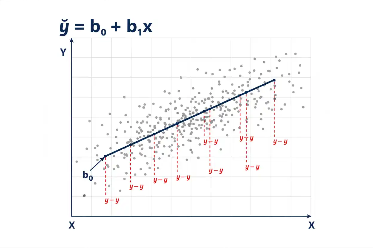
Linear regression is a statistical method used to model how a quantitative response variable changes in relation to one or more explanatory variables. In simple linear regression, one predictor x is used to explain or predict a response y through a straight-line equation of the form ŷ = b₀ + b₁x. The slope b₁ describes the estimated change in the mean response associated with a one-unit increase in x, while the intercept b₀ gives the fitted response when x = 0. Ordinary least squares chooses the fitted line that minimizes the sum of squared vertical residuals between observed and predicted y values. A linear regression model can be used for description, prediction, and statistical inference, but a strong fitted relationship does not by itself establish causation. Its usefulness depends on whether the relationship is reasonably linear, the error structure is appropriate, observations satisfy the required dependence assumptions, and influential points or extrapolation do not distort interpretation. Measures such as R², residual plots, standard errors, confidence intervals, and prediction intervals help evaluate the fitted model, but no single statistic is sufficient on its own.
Linear regression is one of the central modeling tools within core statistics and the wider Statistics & Probability framework. It connects descriptive concepts such as the mean with measures of association and statistical inference while remaining distinct from curved models such as exponential regression and logarithmic regression.
What Is Linear Regression?
Linear regression models the conditional mean of a quantitative response as a linear function of one or more predictors.
For simple linear regression, the population model is commonly written:
Y = β₀ + β₁X + ε
where:
- Y = response variable
- X = explanatory or predictor variable
- β₀ = population intercept
- β₁ = population slope
- ε = random error term
The corresponding fitted sample equation is:
ŷ = b₀ + b₁x
where:
- ŷ = predicted value of y
- b₀ = estimated intercept
- b₁ = estimated slope
- x = specified predictor value
The fitted line summarizes the estimated average relationship between X and Y.
Individual observations usually do not lie exactly on that line because real data contain natural variation, measurement error, omitted influences, and other unexplained differences.
Simple Linear Regression Formula
The basic fitted equation is:
ŷ = b₀ + b₁x
The least-squares slope is:
b₁ = Σ(xᵢ − x̄)(yᵢ − ȳ) / Σ(xᵢ − x̄)²
The intercept is:
b₀ = ȳ − b₁x̄
where:
- xᵢ = ith predictor value
- yᵢ = ith response value
- x̄ = sample mean of x
- ȳ = sample mean of y
- n = number of paired observations
The numerator of the slope formula measures how x and y vary together.
The denominator measures how much x varies around its own mean.
This makes the fitted slope closely related to covariance, even though covariance itself is not the focus of the regression model.
Why Linear Regression Uses Least Squares
For each observation, linear regression calculates a residual:
eᵢ = yᵢ − ŷᵢ
A residual is the vertical difference between the observed response and the fitted value.
Ordinary least squares chooses b₀ and b₁ to minimize:
SSE = Σ(yᵢ − ŷᵢ)²
or equivalently:
SSE = Σeᵢ²
SSE stands for sum of squared errors or residual sum of squares.
Squaring accomplishes two things.
First, positive and negative residuals do not cancel.
Second, larger residuals receive proportionally greater weight.
The resulting optimization problem has a direct algebraic solution, producing the familiar formulas for b₀ and b₁.
Linear Regression Example
Consider the paired data:
| x | y |
|---|---|
| 1 | 2 |
| 2 | 3 |
| 3 | 5 |
| 4 | 4 |
| 5 | 6 |
We want to fit the simple linear regression model:
ŷ = b₀ + b₁x
Step 1: Calculate the Means
For x:
x̄ = (1 + 2 + 3 + 4 + 5)/5
x̄ = 3
For y:
ȳ = (2 + 3 + 5 + 4 + 6)/5
ȳ = 4
Step 2: Calculate Deviations and Cross-Products
| x | y | x − x̄ | y − ȳ | (x − x̄)(y − ȳ) | (x − x̄)² |
|---|---|---|---|---|---|
| 1 | 2 | −2 | −2 | 4 | 4 |
| 2 | 3 | −1 | −1 | 1 | 1 |
| 3 | 5 | 0 | 1 | 0 | 0 |
| 4 | 4 | 1 | 0 | 0 | 1 |
| 5 | 6 | 2 | 2 | 4 | 4 |
Therefore:
Σ(xᵢ − x̄)(yᵢ − ȳ) = 9
and:
Σ(xᵢ − x̄)² = 10
Step 3: Calculate the Slope
b₁ = 9/10
b₁ = 0.9
Step 4: Calculate the Intercept
b₀ = ȳ − b₁x̄
b₀ = 4 − (0.9)(3)
b₀ = 1.3
The fitted linear regression equation is:
ŷ = 1.3 + 0.9x
Interpreting the Slope
The fitted slope is:
b₁ = 0.9
This means that for every one-unit increase in x, the model predicts an average increase of:
0.9 units
in y.
The word average matters.
The slope does not imply that every individual observation increases by exactly 0.9 units whenever x increases by one.
Linear regression describes the fitted conditional mean pattern.
The observed data can vary above and below that line.
Interpreting the Intercept
The fitted intercept is:
b₀ = 1.3
Therefore, when:
x = 0
the regression model predicts:
ŷ = 1.3
Whether this has substantive meaning depends on the context.
If x = 0 is plausible and near the observed data range, the intercept may be meaningful.
If the observations only cover:
100 ≤ x ≤ 200
then interpreting the fitted response at x = 0 would require extreme extrapolation and may be meaningless even though the intercept is mathematically necessary.
Calculating Predicted Values
Using:
ŷ = 1.3 + 0.9x
the predicted response for:
x = 4
is:
ŷ = 1.3 + 0.9(4)
ŷ = 1.3 + 3.6
ŷ = 4.9
The observed response at x = 4 is:
y = 4
Therefore, the prediction error for that observation is:
4 − 4.9 = −0.9
That value is the residual.
Predicted Values for the Full Example
The fitted values are:
| x | Observed y | Predicted ŷ |
|---|---|---|
| 1 | 2 | 2.2 |
| 2 | 3 | 3.1 |
| 3 | 5 | 4.0 |
| 4 | 4 | 4.9 |
| 5 | 6 | 5.8 |
The fitted line does not pass through every observation.
Ordinary least squares instead finds the straight line with the smallest total squared vertical error among all possible straight lines.
Residuals in Linear Regression
Residuals are:
eᵢ = yᵢ − ŷᵢ
For the example:
| x | y | ŷ | Residual e |
|---|---|---|---|
| 1 | 2 | 2.2 | −0.2 |
| 2 | 3 | 3.1 | −0.1 |
| 3 | 5 | 4.0 | 1.0 |
| 4 | 4 | 4.9 | −0.9 |
| 5 | 6 | 5.8 | 0.2 |
A positive residual means:
observed y > predicted y
A negative residual means:
observed y < predicted y
For example, at x = 3:
e = 5 − 4
e = 1
so the observation lies one unit above the fitted line.
Sum of Residuals
When an ordinary least-squares regression includes an intercept, an important property is:
Σeᵢ = 0
apart from numerical rounding.
For the example:
−0.2 − 0.1 + 1.0 − 0.9 + 0.2 = 0
This occurs because the fitted line balances positive and negative residuals in a particular least-squares sense.
However, the fact that residuals sum to zero does not mean the model fits perfectly.
Large positive and negative residuals could still cancel.
That is why least squares works with:
Σeᵢ²
rather than merely:
Σeᵢ
Residual Sum of Squares
For the example:
SSE = Σeᵢ²
Therefore:
SSE = (−0.2)² + (−0.1)² + (1.0)² + (−0.9)² + (0.2)²
SSE = 0.04 + 0.01 + 1 + 0.81 + 0.04
SSE = 1.90
This quantity measures the variation in y that remains unexplained by the fitted line.
Smaller SSE means the fitted values are closer to the observations on the response scale.
However, SSE depends on both measurement units and sample size, so it is not usually meaningful to compare raw SSE values across unrelated data sets without context.
The Regression Line Passes Through the Means
A fitted simple ordinary least-squares regression line with an intercept always passes through:
(x̄, ȳ)
For the example:
x̄ = 3
ȳ = 4
Substitute x = 3 into:
ŷ = 1.3 + 0.9x
Then:
ŷ = 1.3 + 0.9(3)
ŷ = 4
Therefore, the fitted line passes through:
(3, 4)
This follows directly from:
b₀ = ȳ − b₁x̄
Relationship Between Slope and Covariance
The sample covariance is:
sₓᵧ = Σ(xᵢ − x̄)(yᵢ − ȳ)/(n − 1)
and the sample variance of x is:
sₓ² = Σ(xᵢ − x̄)²/(n − 1)
Therefore:
b₁ = sₓᵧ/sₓ²
The n − 1 factors cancel.
This provides another interpretation of the slope.
It measures how strongly x and y vary together relative to the amount of variation available in x.
If covariance is positive, the slope is positive.
If covariance is negative, the slope is negative.
If covariance is zero and Var(X) > 0, the fitted slope is zero.
Linear Regression and Correlation
For simple linear regression with an intercept, the slope is also related to the Pearson correlation coefficient r:
b₁ = r(sᵧ/sₓ)
This means the sign of the slope and the sign of r are always the same.
If:
r > 0
then:
b₁ > 0
If:
r < 0
then:
b₁ < 0
The correlation coefficient is standardized and unitless.
The regression slope is not.
Its units are:
units of y per unit of x
This makes the slope more directly useful for prediction and substantive interpretation.
R² in Linear Regression
The coefficient of determination is commonly written:
R²
It measures the proportion of sample variation in y around its mean that is accounted for by the fitted regression model.
The total sum of squares is:
SST = Σ(yᵢ − ȳ)²
The residual sum of squares is:
SSE = Σ(yᵢ − ŷᵢ)²
Then:
R² = 1 − SSE/SST
For the example:
SST = (2 − 4)² + (3 − 4)² + (5 − 4)² + (4 − 4)² + (6 − 4)²
SST = 4 + 1 + 1 + 0 + 4
SST = 10
Since:
SSE = 1.9
we obtain:
R² = 1 − 1.9/10
R² = 0.81
Therefore:
R² = 81%
About 81% of the observed sample variation in y around its mean is accounted for by the fitted linear relationship with x.
R² and Correlation in Simple Linear Regression
For simple ordinary least-squares regression with one predictor and an intercept:
R² = r²
For the example:
r = 0.9
Therefore:
r² = 0.81
which matches:
R² = 0.81
This equality is specific to simple linear regression with an intercept.
It should not be generalized blindly to every regression model.
R² also should not be interpreted as the percentage of y caused by x.
It is a measure of fitted variation explained within the sample model.
Explained Sum of Squares
The fitted variation can be written:
SSR = Σ(ŷᵢ − ȳ)²
where SSR is the regression sum of squares.
For ordinary least squares with an intercept:
SST = SSR + SSE
For the example:
SST = 10
SSE = 1.9
so:
SSR = 10 − 1.9
SSR = 8.1
Then:
R² = SSR/SST
R² = 8.1/10
R² = 0.81
Both formulas produce the same result.
What Does R² = 0 Mean?
In simple linear regression with an intercept:
R² = 0
means the fitted line does not reduce squared prediction error relative to using the sample mean ȳ for every observation.
In that situation:
b₁ = 0
and the fitted model becomes:
ŷ = ȳ
However, R² = 0 does not imply that x and y are completely unrelated.
A strong nonlinear relationship can have little linear explanatory power.
For example, a symmetric curved relationship can produce a slope near zero.
What Does R² = 1 Mean?
If:
R² = 1
then:
SSE = 0
and every observed point lies exactly on the fitted regression line.
Therefore:
yᵢ = ŷᵢ
for every observation.
This represents perfect in-sample linear fit.
It does not necessarily prove that the relationship will remain exact in new data or that x causes y.
A perfect fit can also occur artificially in very small or overstructured data sets.
Linear Regression vs Mean-Only Prediction
Without a predictor, a natural constant prediction is the mean:
ŷ = ȳ
Linear regression improves on that baseline when x contains useful linear predictive information.
R² compares these two levels of squared error.
If the fitted regression does not perform better than the mean-only baseline under an ordinary intercept model, R² will not be positive.
This connection helps explain why the sample mean is central to regression decomposition.
Standard Error of the Regression
Under the classical simple linear regression framework, the residual variance is estimated using:
s² = SSE/(n − 2)
The denominator is:
n − 2
because two parameters have been estimated:
b₀
and:
b₁
The residual standard error is:
s = √[SSE/(n − 2)]
For the example:
SSE = 1.9
n = 5
Therefore:
s² = 1.9/3
s² ≈ 0.6333
and:
s ≈ 0.7958
This quantity estimates the typical residual spread around the fitted line under the model assumptions.
Standard Error of the Slope
The estimated standard error of b₁ in simple linear regression is:
SE(b₁) = s / √[Σ(xᵢ − x̄)²]
where:
s = √[SSE/(n − 2)]
For the example:
s ≈ 0.7958
and:
Σ(xᵢ − x̄)² = 10
Therefore:
SE(b₁) ≈ 0.7958/√10
SE(b₁) ≈ 0.2517
The slope estimate:
b₁ = 0.9
is therefore subject to noticeable uncertainty because the sample contains only five observations.
Hypothesis Test for the Slope
A common inferential question is:
H₀: β₁ = 0
against:
H₁: β₁ ≠ 0
The test statistic is:
t = (b₁ − 0)/SE(b₁)
For the example:
t ≈ 0.9/0.2517
t ≈ 3.576
The degrees of freedom are:
df = n − 2
df = 3
The observed statistic is compared with a t reference distribution.
Formal decisions then depend on the chosen significance level and corresponding reference-distribution cutoff.
Statistical significance of the slope indicates evidence of nonzero linear association under the model assumptions. It does not automatically imply practical importance or causation.
Confidence Interval for the Slope
A confidence interval for β₁ commonly has the form:
b₁ ± t*SE(b₁)
For a two-sided 95% interval with:
df = 3
the relevant t critical value is approximately:
t* ≈ 3.182
Using:
b₁ = 0.9
and:
SE(b₁) ≈ 0.2517
the margin of error is:
ME ≈ 3.182 × 0.2517
ME ≈ 0.801
Therefore:
Lower bound ≈ 0.9 − 0.801 = 0.099
Upper bound ≈ 0.9 + 0.801 = 1.701
So the approximate interval is:
95% CI ≈ (0.099, 1.701)
The interval is wide because the sample is very small.
This demonstrates why an estimated slope should not be interpreted without considering uncertainty.
Confidence Interval vs Prediction Interval
Linear regression can produce both confidence intervals and prediction intervals, but they answer different questions.
A confidence interval for the mean response at x₀ estimates:
E(Y|X = x₀)
A prediction interval estimates a new individual response at x₀.
Prediction intervals are wider because they account for both:
- uncertainty in estimating the mean response, and
- individual residual variation around that mean.
For a simple linear model, the mean-response standard error includes a term related to:
1/n + (x₀ − x̄)²/Σ(xᵢ − x̄)²
while a prediction interval adds another:
1
inside the variance expression to represent individual outcome variation.
Why Prediction Is Most Precise Near x̄
The uncertainty in the fitted mean response is smallest near:
x = x̄
because:
(x₀ − x̄)²
is smallest there.
As x₀ moves farther from the center of the observed predictor data, uncertainty increases.
This is why regression predictions near the center of the observed x range are generally more stable than predictions near its extremes.
It also helps explain why extrapolation is particularly uncertain.
Interpolation vs Extrapolation
Interpolation predicts y for x values inside the observed predictor range.
Extrapolation predicts outside that range.
In the example, observed x values are:
1 through 5
Predicting at:
x = 3.5
is interpolation.
Predicting at:
x = 20
is extrapolation.
The fitted equation can mechanically generate both predictions, but that does not make them equally credible.
A relationship that appears linear over x = 1 to 5 may change substantially by x = 20.
Extrapolation requires substantive justification beyond the regression formula.
Linearity Assumption
Simple linear regression assumes the conditional mean of Y is appropriately represented by a straight line:
E(Y|X=x) = β₀ + β₁x
This does not require every observation to lie on a line.
It requires the systematic average relationship to be linear.
A residual plot can help assess this assumption.
If residuals show a strong U-shape, arch, or other systematic curve, the linear model may be misspecified.
A curved model such as logarithmic regression or exponential regression may then better describe the relationship if supported by the data and subject matter.
Independence Assumption
Classical linear regression often assumes that error terms are independent across observations.
This can fail with:
- repeated measurements,
- time-series data,
- clustered observations,
- family or household data,
- students within the same classrooms,
- measurements from the same experimental unit.
If observations are dependent, ordinary least-squares coefficient estimates may still sometimes have useful properties, but conventional standard errors and inference can become incorrect.
Dependence should therefore be addressed through the study design or an appropriate statistical model rather than ignored.
Constant Variance Assumption
A common classical assumption is:
Var(ε|X=x) = σ²
for all relevant x.
This is called homoscedasticity.
If residual spread increases or decreases systematically with x or ŷ, the data exhibit heteroscedasticity.
For example, a residual plot shaped like a funnel suggests changing variance.
Heteroscedasticity does not automatically make the fitted slope meaningless, but conventional standard errors, confidence intervals, and tests may become unreliable unless the issue is handled appropriately.
Normality Assumption
Normality is often misunderstood in linear regression.
Ordinary least squares does not require x or y themselves to be normally distributed simply to calculate b₀ and b₁.
Classical small-sample t and F inference is commonly derived under an assumption that model errors are normally distributed conditional on X.
With larger samples, some inference can be robust to moderate non-normality under suitable conditions.
However, severe outliers, heavy tails, dependence, or model misspecification can still create substantial problems.
The relevant concern is the behavior of errors under the model, not whether every raw variable has a bell-shaped histogram.
Zero Conditional Mean Assumption
A fundamental regression condition is commonly expressed as:
E(ε|X) = 0
This means the predictor is not systematically associated with omitted influences contained in the error term.
If this condition fails, the fitted slope can be biased for the causal or structural relationship of interest.
For example, an omitted variable that affects Y and is correlated with X can create omitted-variable bias.
This issue is especially important when regression coefficients are interpreted causally rather than merely descriptively.
Regression and Causation
Linear regression measures conditional association.
It does not automatically establish:
X causes Y
A statistically significant slope can arise because of:
- genuine causal influence,
- reverse causation,
- confounding,
- selection effects,
- common trends,
- measurement structure,
- chance under model uncertainty.
Causal interpretation requires additional assumptions and often a research design such as random assignment, credible natural experiments, or carefully justified causal modeling.
The regression equation alone cannot distinguish association from causation.
Outliers in Linear Regression
An outlier is an observation with an unusual value relative to some aspect of the data.
An unusual y value can produce a large residual.
A predictor value far from the bulk of the x observations can have high leverage.
Some observations can be both unusual and highly influential.
A simple descriptive rule based on the interquartile range can flag extreme univariate values, but regression influence depends on the joint x-y structure.
An observation should therefore not be removed solely because it lies beyond an IQR fence.
Its data quality, leverage, residual, influence, and substantive context should be examined.
Leverage
Leverage describes how unusual an observation’s predictor value is relative to the rest of the data.
In simple linear regression, leverage increases as:
|xᵢ − x̄|
increases.
A point far from the center of the predictor distribution can strongly affect the fitted line because relatively few other observations anchor the line in that region.
High leverage is not automatically problematic.
An observation can have high leverage and still lie close to the overall regression trend.
Concern becomes greater when high leverage is combined with a substantial residual.
Influential Observations
An influential observation materially changes the fitted regression when included or excluded.
Influence depends on a combination of:
- residual size,
- leverage,
- sample size,
- overall data configuration.
Measures such as Cook’s distance can help identify influential observations.
However, influence diagnostics are investigative tools rather than automatic deletion rules.
A highly influential point may represent an important part of the population and should not be removed merely because it changes the estimated slope.
Residual Plots
A residual plot typically places residuals on the vertical axis and x or fitted values on the horizontal axis.
A well-behaved simple linear regression often shows residuals scattered roughly around:
0
without obvious systematic pattern.
Potential warning signs include:
- curved patterns,
- funnel-shaped spread,
- clusters,
- isolated extreme residuals,
- temporal sequences,
- abrupt structural changes.
A residual plot does not prove every assumption, but it can reveal problems hidden by R² or the slope estimate alone.
Linear Regression vs Exponential Regression
Linear regression models constant additive change.
A simple linear equation has:
ŷ = b₀ + b₁x
For every one-unit increase in x, the fitted response changes by:
b₁
units.
Exponential regression instead commonly has:
ŷ = abˣ
For every one-unit increase in x, the fitted response is multiplied by:
b
The distinction is:
Linear regression → constant difference
Exponential regression → constant ratio
A curved upward pattern that accelerates may therefore require an exponential rather than linear model if the underlying structure supports multiplicative growth.
Linear Regression vs Logarithmic Regression
A logarithmic regression commonly has the form:
ŷ = a + b ln(x)
with:
x > 0
This model changes rapidly at smaller x values and then gradually flattens as x increases.
Linear regression instead assumes:
ŷ = b₀ + b₁x
with a constant slope.
The appropriate choice should follow the data pattern and substantive mechanism.
A strong R² alone should not determine which equation is preferable if the competing models imply very different behavior outside the observed range.
Linear Regression and Geometric Distribution
The geometric distribution models discrete waiting times until a first success.
Linear regression models the conditional mean of a response in relation to predictors.
These are fundamentally different statistical objects.
A geometric random variable is:
discrete
positive
usually right-skewed
and governed by a success probability p.
Ordinary linear regression does not automatically provide an appropriate model for such waiting-time outcomes.
Specialized generalized modeling may be needed when the response follows a discrete probability structure.
Linear Regression With Multiple Predictors
Multiple linear regression extends the model to several explanatory variables:
Y = β₀ + β₁X₁ + β₂X₂ + … + βₖXₖ + ε
The fitted equation is:
ŷ = b₀ + b₁x₁ + b₂x₂ + … + bₖxₖ
Each coefficient is interpreted as the estimated change in the mean response associated with a one-unit increase in that predictor holding the other included predictors constant.
This conditional interpretation differs from the simple bivariate relationship.
Adding predictors can help adjust for measured factors, but it does not automatically eliminate confounding or establish causation.
Linear in Parameters Does Not Always Mean a Straight Line
The term linear regression refers fundamentally to linearity in the model coefficients, not necessarily to a straight-line graph in every predictor representation.
For example:
Y = β₀ + β₁X + β₂X² + ε
is linear in:
β₀, β₁, β₂
even though the fitted relationship between X and Y is curved.
Polynomial regression can therefore be estimated using linear least-squares machinery.
The specialist focus here remains the simple straight-line case:
ŷ = b₀ + b₁x
because that is the core linear regression model.
Dummy Variables in Linear Regression
Categorical predictors can be included in linear regression through indicator variables.
Suppose a variable has two groups.
Define:
D = 0 for Group A
D = 1 for Group B
Then:
Y = β₀ + β₁D + ε
gives:
Group A mean = β₀
and:
Group B mean = β₀ + β₁
Therefore:
β₁
represents the difference between the group means.
This illustrates how linear regression can encompass comparisons that may at first seem different from ordinary straight-line prediction.
Interaction Terms
A regression model can also allow the effect of one predictor to depend on another.
For example:
Y = β₀ + β₁X + β₂D + β₃XD + ε
The product:
XD
is an interaction term.
If D identifies two groups, the slope for one group can differ from the slope for the other.
The presence of an interaction changes the interpretation of the individual coefficients.
A coefficient should therefore never be interpreted in isolation without considering the full model containing it.
Regression Coefficients Depend on Units
Suppose x is measured in meters and the fitted slope is:
b₁ = 5
units of y per meter.
If x is converted to centimeters, a one-centimeter change is:
1/100
of a meter.
The numerical slope becomes:
0.05
units of y per centimeter.
The underlying relationship has not changed.
Regression slopes therefore depend on measurement units.
This differs from the standardized correlation coefficient, which is invariant to positive linear unit changes.
Standardized Regression Coefficients
Variables can be standardized:
Zₓ = (X − x̄)/sₓ
Zᵧ = (Y − ȳ)/sᵧ
In simple linear regression of standardized Y on standardized X, the slope equals the Pearson correlation coefficient:
bstandardized = r
This provides another mathematical link between regression and correlation.
However, standardized coefficients can be less directly interpretable in real measurement units.
A slope such as:
2.5 kilograms per centimeter
may be more practically meaningful than a standardized coefficient when substantive interpretation is the goal.
Linear Regression and Statistical Significance
A statistically significant slope does not mean the fitted model is necessarily useful.
A sufficiently large sample can detect a very small slope.
For example:
b₁ = 0.002
might produce a very small p-value if its standard error is tiny.
Whether a 0.002-unit change matters depends on the variables and application.
Conversely, a substantively important slope can fail to reach statistical significance in a small sample because uncertainty is large.
Statistical significance and practical significance must therefore be evaluated separately.
R² Does Not Measure Causation
Suppose:
R² = 0.90
This means the fitted linear model accounts for 90% of the sample variation in y around ȳ under the usual decomposition.
It does not mean:
x causes 90% of y
or:
90% of y is caused by x.
High R² can arise from common trends, confounding, data construction, or other noncausal mechanisms.
Causal conclusions require a defensible research design and assumptions beyond goodness of fit.
A High R² Does Not Guarantee a Good Model
A high R² can coexist with:
- nonlinear residual patterns,
- influential outliers,
- extrapolation problems,
- omitted-variable bias,
- dependence,
- heteroscedasticity,
- poor causal interpretation.
For example, two variables that both increase over time can show an extremely high R² even if one does not meaningfully explain the other.
Residual diagnostics and substantive reasoning remain necessary.
R² is useful, but it is not a complete model-quality score.
A Low R² Does Not Always Mean the Model Is Useless
In fields with substantial individual variability, even meaningful relationships can have modest R² values.
Suppose:
R² = 0.15
A predictor may still be strongly associated with the response in a scientifically important way.
Low R² means much of the sample variation remains unexplained by the fitted model.
It does not automatically mean the slope is zero or useless.
Predictive usefulness depends on the required accuracy and application.
Inferential usefulness can also exist even when prediction at the individual level remains imprecise.
Overfitting
Overfitting occurs when a model captures random peculiarities of the observed sample rather than stable structure that generalizes.
Simple linear regression with one predictor has relatively limited flexibility, but overfitting becomes more important as predictors, transformations, interactions, or polynomial terms are added.
A model can fit existing data extremely well yet perform poorly on new observations.
Out-of-sample validation and substantive simplicity become increasingly important as model complexity grows.
The purpose is not merely to maximize in-sample R².
Prediction vs Explanation
Linear regression can be used for different goals.
A predictive model asks:
How accurately can y be predicted for new observations?
An explanatory or inferential model asks:
How is y associated with x, and what does the slope tell us about the underlying population relationship?
A causal model asks an even stronger question:
What would happen to y if x were changed through an intervention?
These goals require different assumptions and evaluation criteria.
A model that predicts well may not identify causal effects, and a causal model may not maximize pure predictive accuracy.
Linear Regression and Missing Data
Ordinary regression requires values for all variables used in a given fitted observation.
If data are missing, simply analyzing complete cases can reduce sample size and can create bias if missingness is related to the variables or outcomes.
Missing values should not automatically be replaced with:
0
because zero is usually a legitimate numerical value rather than a marker for missingness.
The appropriate handling depends on why data are missing and on the statistical model.
Missing-data decisions can materially affect slopes, standard errors, and predictions.
Linear Regression and Measurement Error
Measurement error in y typically increases residual variability.
Measurement error in x can create more complicated problems.
In the classical simple case, random measurement error in the predictor can bias the estimated slope toward zero, a phenomenon often called attenuation.
Therefore, precisely measuring the predictor can be important for valid interpretation.
Ordinary least squares usually treats observed x values as known without error within the basic model.
When predictor measurement error is substantial, specialized methods may be necessary.
Common Linear Regression Mistakes
A common mistake is interpreting the slope as causal simply because it is statistically significant.
Another is extrapolating far beyond the observed x range without evidence that the linear pattern continues.
A third mistake is judging the model solely by R².
Analysts also sometimes ignore residual plots, making it easy to miss strong curvature or changing variance.
Another error is assuming raw x or y data must be normally distributed. The classical inferential assumptions concern the error structure rather than requiring both observed variables to have normal marginal distributions.
It is also incorrect to interpret the intercept literally when x = 0 lies far outside the meaningful or observed range.
Removing observations solely because they are unusual under an interquartile range rule can also distort the regression.
Finally, confusing linear regression with curved models can lead to poor predictions when the actual relationship follows multiplicative or logarithmic change.
How to Calculate Linear Regression Step by Step
A reliable simple linear regression calculation follows this sequence.
Step 1: Arrange Paired Observations
Write the data as:
(x₁, y₁), (x₂, y₂), …, (xₙ, yₙ)
Each x value must correspond to the correct y observation.
Step 2: Calculate the Means
x̄ = Σxᵢ/n
ȳ = Σyᵢ/n
Step 3: Calculate the Slope Numerator
Sxy = Σ(xᵢ − x̄)(yᵢ − ȳ)
Step 4: Calculate the Slope Denominator
Sxx = Σ(xᵢ − x̄)²
Step 5: Calculate the Slope
b₁ = Sxy/Sxx
Step 6: Calculate the Intercept
b₀ = ȳ − b₁x̄
Step 7: Write the Fitted Equation
ŷ = b₀ + b₁x
Step 8: Calculate Fitted Values
For each x:
ŷᵢ = b₀ + b₁xᵢ
Step 9: Calculate Residuals
eᵢ = yᵢ − ŷᵢ
Step 10: Evaluate the Model
Examine residuals, R², uncertainty, outliers, assumptions, and whether the relationship is substantively reasonable.
How to Report a Linear Regression
A useful report should communicate more than the equation alone.
For the worked example:
ŷ = 1.3 + 0.9x
A direct interpretation is:
Each one-unit increase in x is associated with an estimated 0.9-unit increase in the mean response y.
The model has:
R² = 0.81
so approximately 81% of the observed sample variation in y around its mean is accounted for by the fitted straight-line relationship.
If formal inference is required, the result should additionally include the slope standard error, confidence interval, test statistic, degrees of freedom, and p-value.
The language should describe association unless the study design genuinely supports a causal interpretation.
Frequently Asked Questions About Linear Regression
What is linear regression?
Linear regression is a statistical method that models a quantitative response as a linear function of one or more explanatory variables.
What is the simple linear regression formula?
The fitted equation is:
ŷ = b₀ + b₁x
where b₀ is the intercept and b₁ is the slope.
What is the slope formula?
For simple ordinary least squares:
b₁ = Σ(xᵢ − x̄)(yᵢ − ȳ) / Σ(xᵢ − x̄)²
What is the intercept formula?
b₀ = ȳ − b₁x̄
What does the slope mean?
The slope represents the estimated change in the mean response y associated with a one-unit increase in x.
What does the intercept mean?
The intercept is the predicted response when:
x = 0
Its practical interpretation depends on whether x = 0 is meaningful and within a reasonable range of the data.
What is a residual?
A residual is:
eᵢ = yᵢ − ŷᵢ
It measures the vertical difference between an observed response and its fitted value.
What does ordinary least squares minimize?
It minimizes:
SSE = Σ(yᵢ − ŷᵢ)²
the sum of squared residuals.
What is R²?
R² is the proportion of sample variation in y around its mean accounted for by the fitted regression model:
R² = 1 − SSE/SST
Is R² the same as correlation squared?
In simple ordinary least-squares regression with one predictor and an intercept:
R² = r²
This equality does not apply universally to every regression setup.
Does a high R² prove causation?
No. R² measures in-sample goodness of fit, not causal influence.
Can linear regression have a negative slope?
Yes. A negative slope means larger x values are associated with smaller fitted mean y values.
Can the slope equal zero?
Yes. A zero slope produces a horizontal fitted line:
ŷ = b₀
and indicates no fitted linear change in y as x changes.
Does linear regression require normal x values?
No. The predictor itself does not need to follow a normal distribution for ordinary least-squares coefficients to be calculated.
Does linear regression require normal y values?
Not directly. Classical exact small-sample inference is commonly based on assumptions concerning the model errors conditional on x rather than requiring the marginal y distribution itself to be normal.
What is homoscedasticity?
Homoscedasticity means the conditional error variance is constant:
Var(ε|X=x) = σ²
across the relevant predictor range.
What is heteroscedasticity?
Heteroscedasticity occurs when residual or error variance changes systematically with x or the fitted response.
What is the difference between linear regression and correlation?
Correlation measures standardized linear association symmetrically between two variables. Regression models a response as a function of predictors and produces coefficients in the variables’ measurement units.
What is the difference between linear and exponential regression?
Linear regression models constant additive change:
ŷ = b₀ + b₁x
Exponential regression models constant multiplicative change:
ŷ = abˣ
What is the difference between linear and logarithmic regression?
Linear regression assumes a constant slope. Logarithmic regression commonly uses:
ŷ = a + b ln(x)
and describes change that is often rapid initially and then progressively slower.
Can linear regression be used for prediction?
Yes. The fitted equation can predict the mean response or future observations, but uncertainty should be quantified and extrapolation beyond the observed predictor range should be treated cautiously.
What is the difference between a confidence interval and a prediction interval in regression?
A confidence interval estimates uncertainty around the mean response. A prediction interval accounts for both uncertainty in the mean response and the additional variability of a future individual observation, so it is wider.
Does statistical significance mean the regression is important?
No. A slope can be statistically significant but practically tiny, particularly in a very large sample.
Can outliers affect linear regression?
Yes. Some unusual observations can substantially alter the slope, intercept, R², and inference, especially when they also have high leverage.
Should unusual observations automatically be deleted?
No. They should be investigated for data quality, leverage, influence, and substantive relevance before any exclusion decision.
What is multiple linear regression?
Multiple linear regression extends the model to several predictors:
ŷ = b₀ + b₁x₁ + b₂x₂ + … + bₖxₖ
Each coefficient describes an adjusted association conditional on the other included predictors.
Does linear regression prove that x causes y?
No. Regression by itself describes association. Causal conclusions require additional design and assumptions about confounding, selection, measurement, and the data-generating process.




