


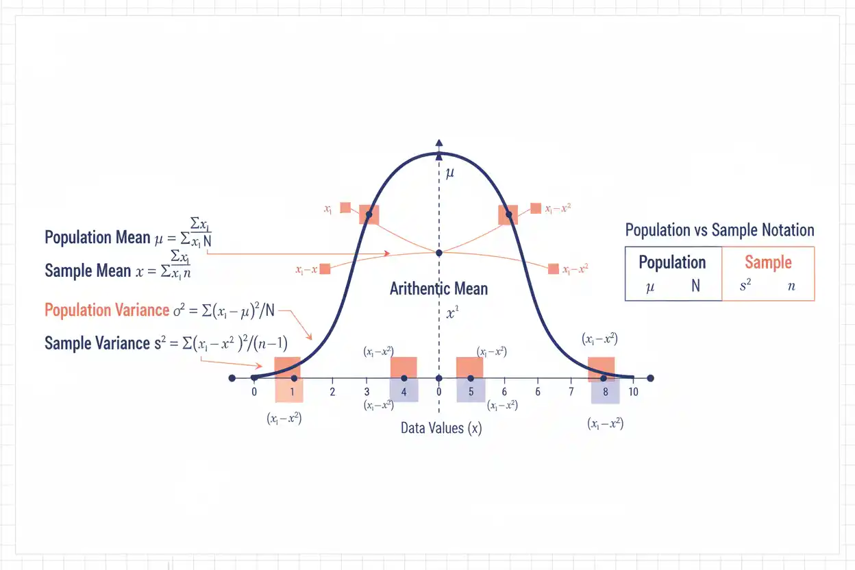
Mean and variance are two fundamental statistical measures used together to describe the center and spread of numerical data or a probability distribution. The mean identifies the arithmetic center or expected value, while the variance measures the average squared distance of values from that center. Two data sets can have exactly the same mean but radically different variance, which is why center alone cannot describe how observations are distributed. For a complete population, variance is calculated by averaging squared deviations from the population mean, whereas the conventional sample variance uses n − 1 in the denominator when estimating population variance from sample data. Variance is always nonnegative and is expressed in squared measurement units, while its square root—the standard deviation—returns dispersion to the original units. In probability theory, mean and variance are often written as E(X) and Var(X), and the identity Var(X) = E(X²) − [E(X)]² provides a useful alternative calculation. Together, mean and variance form the foundation for probability distributions, statistical inference, regression, sampling theory, risk analysis, and many other quantitative methods.
Within core statistics, mean and variance provide complementary information: one identifies where values are centered, while the other describes how widely they vary around that center. They belong to the broader Statistics & Probability framework and connect directly with the arithmetic mean, while comparisons among different measures of center are handled separately in mean, median, mode.
What Are Mean and Variance?
The mean summarizes central location.
The variance summarizes squared dispersion around that mean.
For a set of numerical observations, the basic logic is:
Mean → Where is the center?
Variance → How far are values spread around that center?
Suppose two data sets are:
A: 8, 9, 10, 11, 12
and:
B: 0, 5, 10, 15, 20
Both have mean:
10
However, the values in B are much farther from 10 than the values in A.
Therefore:
Mean(A) = Mean(B)
but:
Variance(B) > Variance(A)
This illustrates why mean and variance are commonly considered together.
Mean Formula
For sample observations:
x₁, x₂, …, xₙ
the sample mean is:
x̄ = Σxᵢ/n
where:
- x̄ = sample mean
- xᵢ = individual observation
- n = sample size
For a finite population:
μ = Σxᵢ/N
where:
- μ = population mean
- N = population size
The calculation is structurally identical.
The notation distinguishes whether the values represent a sample or the complete population of interest.
The dedicated mean page develops the arithmetic average in greater detail; here the focus is how the mean functions as the reference point for variance.
Population Variance Formula
For a finite population, variance is:
σ² = Σ(xᵢ − μ)²/N
where:
- σ² = population variance
- xᵢ = population observation
- μ = population mean
- N = population size
The calculation has four basic stages:
- Find the population mean.
- Subtract the mean from every observation.
- Square each deviation.
- Average those squared deviations.
The result measures the average squared distance from the population mean.
Sample Variance Formula
For sample observations used to estimate population variance, the conventional sample variance is:
s² = Σ(xᵢ − x̄)²/(n − 1)
where:
- s² = sample variance
- x̄ = sample mean
- n = sample size
The denominator is:
n − 1
rather than:
n
because the sample mean has been estimated from the same observations.
This adjustment gives the familiar unbiased estimator of population variance under standard independent sampling assumptions with finite variance.
Population vs Sample Variance
The distinction is important.
For a complete population:
σ² = Σ(xᵢ − μ)²/N
For a sample estimating a larger population:
s² = Σ(xᵢ − x̄)²/(n − 1)
Using n in the second expression produces the average squared deviation around the sample mean for the observed sample itself, but it is downward biased as an estimator of the population variance under the conventional sampling framework.
Therefore:
Population description → divide by N
Conventional sample variance estimator → divide by n − 1
The correct formula depends on the statistical role of the data.
Mean and Variance Example
Consider:
2, 4, 6, 8, 10
We will calculate both the mean and variance.
Step 1: Find the Mean
x̄ = (2 + 4 + 6 + 8 + 10)/5
x̄ = 30/5
x̄ = 6
Therefore:
Mean = 6
Step 2: Calculate Deviations
| x | x − 6 |
|---|---|
| 2 | −4 |
| 4 | −2 |
| 6 | 0 |
| 8 | 2 |
| 10 | 4 |
The signed deviations sum to:
−4 − 2 + 0 + 2 + 4 = 0
This always occurs for deviations from the arithmetic sample mean.
Step 3: Square the Deviations
| x | x − 6 | (x − 6)² |
|---|---|---|
| 2 | −4 | 16 |
| 4 | −2 | 4 |
| 6 | 0 | 0 |
| 8 | 2 | 4 |
| 10 | 4 | 16 |
The sum of squared deviations is:
16 + 4 + 0 + 4 + 16 = 40
Step 4: Calculate Population Variance
If these five values are the complete population:
σ² = 40/5
σ² = 8
Therefore:
Population mean = 6
Population variance = 8
Step 5: Calculate Sample Variance
If the same five values are a sample from a larger population:
s² = 40/(5 − 1)
s² = 40/4
s² = 10
Therefore:
Sample mean = 6
Sample variance = 10
The observed data are identical; only their statistical interpretation changes the variance denominator.
Why Variance Uses Squared Deviations
If ordinary deviations were averaged:
Σ(xᵢ − x̄)/n
the result would always be:
0
because positive and negative deviations cancel.
Squaring prevents that cancellation:
(−4)² = 16
4² = 16
Both observations contribute equally when they are equally far from the mean.
Squaring also gives greater weight to larger deviations.
A deviation of:
2
contributes:
2² = 4
while a deviation of:
10
contributes:
10² = 100
The second deviation is five times farther from the mean but contributes twenty-five times as much squared variation.
Mean Absolute Deviation vs Variance
An alternative measure of spread is mean absolute deviation.
Mean absolute deviation about the arithmetic mean uses:
|xᵢ − x̄|
Variance uses:
(xᵢ − x̄)²
Mean absolute deviation therefore measures average absolute distance.
Variance measures average squared distance.
The two respond differently to extreme observations because squaring amplifies large deviations much more strongly.
For example:
deviation = 3
gives:
absolute deviation = 3
squared deviation = 9
while:
deviation = 12
gives:
absolute deviation = 12
squared deviation = 144
Variance is consequently especially sensitive to extreme values.
Standard Deviation From Variance
Variance is expressed in squared units.
If the variable is measured in:
meters
then variance is measured in:
meters²
Taking the square root gives the standard deviation:
σ = √σ²
for a population, or:
s = √s²
for a sample.
In the worked population example:
σ² = 8
Therefore:
σ = √8
σ ≈ 2.828
For the sample variance:
s² = 10
so:
s = √10
s ≈ 3.162
Standard deviation is often easier to interpret because it returns to the original measurement units.
What Does Variance Mean?
Suppose a population has:
Mean = 20
Variance = 25
The squared dispersion is:
25 units²
The corresponding standard deviation is:
√25 = 5 units
Variance itself is mathematically useful but is often less intuitive in direct verbal interpretation because of its squared units.
Its main role is to quantify dispersion in a form with powerful algebraic properties.
Can Variance Be Negative?
No.
Every squared deviation satisfies:
(xᵢ − μ)² ≥ 0
Therefore:
σ² ≥ 0
and:
s² ≥ 0
A negative variance indicates an error in arithmetic, data processing, or numerical computation.
In exact mathematics, variance can never be less than zero.
When Is Variance Equal to Zero?
Variance equals zero only when every observation is identical.
If:
σ² = 0
then every squared deviation must equal zero:
(xᵢ − μ)² = 0
Therefore:
xᵢ = μ
for every observation.
For example:
7, 7, 7, 7
has:
Mean = 7
Variance = 0
There is no dispersion.
Same Mean, Different Variance
Consider:
Data A: 9, 10, 11
and:
Data B: 0, 10, 20
Both have:
x̄ = 10
For Data A, population squared deviations are:
1, 0, 1
so:
σ²A = 2/3
σ²A ≈ 0.667
For Data B, squared deviations are:
100, 0, 100
so:
σ²B = 200/3
σ²B ≈ 66.667
The means are identical, but Data B is much more dispersed.
This is precisely why mean and variance describe different properties.
Different Mean, Same Variance
Two data sets can also have different centers but identical variance.
Consider:
A: 1, 3, 5
and:
B: 101, 103, 105
Their means are:
Mean(A) = 3
Mean(B) = 103
Yet both have deviations:
−2, 0, 2
around their respective means.
Therefore, their variances are equal.
Changing location does not necessarily change dispersion.
Effect of Adding a Constant
Suppose:
Y = X + c
Then:
E(Y) = E(X) + c
but:
Var(Y) = Var(X)
Adding a constant moves every value and the mean by the same amount.
The deviations remain unchanged:
(X + c) − (μ + c) = X − μ
Therefore, adding a constant changes the mean but leaves variance unchanged.
For example, if a data set has:
Mean = 20
Variance = 9
and 100 is added to every observation, then:
New mean = 120
New variance = 9
Effect of Multiplying by a Constant
Suppose:
Y = aX
Then:
E(Y) = aE(X)
and:
Var(Y) = a²Var(X)
Why is variance multiplied by a²?
Because deviations are multiplied by a:
Y − E(Y) = a[X − E(X)]
Squaring gives:
[Y − E(Y)]² = a²[X − E(X)]²
Therefore, variance scales quadratically.
If all observations are doubled:
Mean doubles
but:
Variance multiplies by 4
If observations are multiplied by 10:
Variance multiplies by 100
General Linear Transformation
For:
Y = aX + b
the mean and variance transform as:
E(Y) = aE(X) + b
and:
Var(Y) = a²Var(X)
The constant b changes location but not dispersion.
The multiplier a changes both.
This pair of formulas is one of the most useful relationships involving mean and variance.
Example of a Linear Transformation
Suppose:
μX = 5
and:
Var(X) = 4
Define:
Y = 3X + 10
Then:
E(Y) = 3(5) + 10
E(Y) = 25
For the variance:
Var(Y) = 3²(4)
Var(Y) = 9(4)
Var(Y) = 36
Therefore:
Mean(Y) = 25
Variance(Y) = 36
The added 10 affects only the mean.
Alternative Variance Formula
Variance can also be calculated using:
Var(X) = E(X²) − [E(X)]²
This is often called the computational or shortcut identity.
For a finite population:
σ² = [Σxᵢ²/N] − μ²
The formula can be easier for theoretical probability calculations.
However, when implemented with floating-point data containing very large values and very small variance, directly subtracting two nearly equal large quantities can cause numerical precision problems.
Centered computational methods are often more stable in software.
Deriving the Variance Identity
Start with:
Var(X) = E[(X − μ)²]
Expand the square:
(X − μ)² = X² − 2μX + μ²
Take expectations:
Var(X) = E(X²) − 2μE(X) + μ²
Since:
E(X) = μ
we obtain:
Var(X) = E(X²) − 2μ² + μ²
Therefore:
Var(X) = E(X²) − μ²
or:
Var(X) = E(X²) − [E(X)]²
This identity appears throughout probability theory.
Shortcut Formula Example
Use the population data:
2, 4, 6, 8, 10
The mean is:
μ = 6
Calculate squared values:
2² + 4² + 6² + 8² + 10²
= 4 + 16 + 36 + 64 + 100
= 220
Therefore:
E(X²) = 220/5
E(X²) = 44
Then:
Var(X) = 44 − 6²
= 44 − 36
= 8
This matches the direct calculation.
Mean and Variance of a Discrete Random Variable
For a discrete random variable X with probability mass function P(X = x):
μ = E(X) = ΣxP(X = x)
Variance is:
Var(X) = Σ(x − μ)²P(X = x)
or equivalently:
Var(X) = E(X²) − μ²
where:
E(X²) = Σx²P(X = x)
This probability-weighted form generalizes the ordinary finite-data calculation.
Values with larger probabilities contribute more strongly.
Discrete Probability Example
Suppose X has:
| x | P(X = x) |
|---|---|
| 0 | 0.25 |
| 1 | 0.50 |
| 2 | 0.25 |
The mean is:
E(X) = 0(0.25) + 1(0.50) + 2(0.25)
E(X) = 1
Now calculate:
E(X²) = 0²(0.25) + 1²(0.50) + 2²(0.25)
E(X²) = 0 + 0.50 + 1
E(X²) = 1.5
Therefore:
Var(X) = 1.5 − 1²
Var(X) = 0.5
So:
Mean = 1
Variance = 0.5
Mean and Variance of a Continuous Random Variable
For a continuous random variable with probability density f(x):
E(X) = ∫xf(x) dx
when the expectation exists.
Variance is:
Var(X) = ∫(x − μ)²f(x) dx
or:
Var(X) = E(X²) − [E(X)]²
provided the relevant integrals are finite.
Thus, mean and variance are not restricted to observed data sets.
They are fundamental properties of probability distributions.
Expected Value Is a Population Mean
In probability theory, the expected value:
E(X)
acts as the theoretical population mean.
It does not necessarily correspond to a value that X can actually take.
For example, a discrete variable might take only:
0 or 1
while having:
E(X) = 0.35
The value 0.35 is still its mean.
It represents the long-run probability-weighted average rather than a required individual outcome.
Variance Measures Expected Squared Deviation
The probability definition:
Var(X) = E[(X − μ)²]
can be read literally as:
expected squared distance from the mean.
This perspective helps unify descriptive data analysis and probability theory.
In observed data, squared deviations are averaged over observations.
In a probability model, squared deviations are averaged using probabilities.
The statistical idea is the same.
Mean and Variance of a Bernoulli Variable
Suppose:
X ~ Bernoulli(p)
with:
P(X = 1) = p
and:
P(X = 0) = 1 − p
The mean is:
E(X) = p
Because:
X² = X
for X ∈ {0,1},
we also have:
E(X²) = p
Therefore:
Var(X) = p − p²
Var(X) = p(1 − p)
This is a fundamental probability result.
Mean and Variance of a Binomial Variable
If:
X ~ Binomial(n, p)
then:
E(X) = np
and:
Var(X) = np(1 − p)
The mean gives the expected number of successes.
The variance quantifies the spread of the success count around that expected value.
For example, if:
n = 20
and:
p = 0.30
then:
E(X) = 20(0.30)
= 6
and:
Var(X) = 20(0.30)(0.70)
= 4.2
The corresponding standard deviation is:
√4.2 ≈ 2.049
Mean and Variance of a Geometric Variable
Using the convention where X counts the trial number of the first success:
E(X) = 1/p
and:
Var(X) = (1 − p)/p²
For:
p = 0.25
the mean is:
E(X) = 4
and:
Var(X) = 0.75/0.0625
= 12
The relatively large variance reflects the possibility of long waiting times.
Different probability distributions can have very different mean–variance relationships.
Mean and Variance of a Negative Binomial Variable
The negative binomial distribution generalizes waiting-count models to a specified number of successes.
Under a common parameterization where X counts the number of trials required to obtain r successes:
E(X) = r/p
and:
Var(X) = r(1 − p)/p²
Other conventions count failures rather than total trials, so formulas and support shift accordingly.
This is another reason parameterization must be checked before applying memorized mean and variance formulas.
Mean–Variance Relationships
Some probability distributions have a fixed relationship between their mean and variance.
For a Bernoulli variable:
Mean = p
Variance = p(1 − p)
For a binomial variable:
Mean = np
Variance = np(1 − p)
For a Poisson variable:
Mean = λ
Variance = λ
For other distributions, the two quantities can vary more independently.
Recognizing these relationships helps identify distributional assumptions and understand dispersion.
Why Mean and Variance Do Not Determine Every Distribution
Knowing only:
E(X)
and:
Var(X)
does not usually identify the complete distribution.
Many different distributions can share the same mean and variance.
For example, a symmetric distribution, a skewed distribution, and a multimodal distribution can potentially have identical first two moments.
Therefore, mean and variance provide essential but incomplete information.
Distribution shape, quantiles, tails, dependence, and other characteristics may also matter.
Mean and Variance in Symmetric Data
For symmetric distributions, the mean often lies at the center when it exists.
Variance then describes how far the distribution spreads around that center in squared-distance terms.
However, two symmetric distributions can have the same mean and variance while differing in tail thickness.
For example, one can place more probability near the center and more probability far into the tails while preserving the same first two moments.
Mean and variance should therefore not be mistaken for a full shape description.
Mean and Variance in Skewed Data
Both measures remain mathematically valid for many skewed distributions as long as the required moments exist.
However, the mean can be pulled toward a long tail, while variance can be strongly influenced by extreme observations.
In highly skewed observed data, it can therefore be useful to inspect robust summaries such as:
- median,
- quartiles,
- interquartile range,
- absolute-deviation measures.
The appropriate summary depends on the question rather than a rule that mean and variance are always either correct or incorrect.
Outliers and Variance
Variance is highly sensitive to extreme observations.
Consider:
2, 4, 6, 8, 10
with population variance:
8
Now replace 10 with:
100
The data become:
2, 4, 6, 8, 100
The new mean is:
24
Squared deviations are:
484, 400, 324, 256, 5,776
Their sum is:
7,240
Population variance becomes:
7,240/5
= 1,448
The variance increases from:
8
to:
1,448
because the extreme value affects both the center and the squared deviations.
Mean and Variance vs Mean Absolute Deviation
Suppose analysts want an intuitive original-unit description of spread.
The mean absolute deviation can provide:
average absolute distance from the mean
Variance instead provides:
average squared distance from the mean
The distinction matters because squared loss disproportionately emphasizes large errors.
Variance is mathematically central in probability and inference, while mean absolute deviation can sometimes be easier to explain descriptively.
Neither measure should be selected simply because it produces the smaller numerical value; their units and definitions differ.
Mean and Variance vs Mean, Median, Mode
Mean and variance should also be distinguished from the broader comparison of mean, median, mode.
Mean, median, and mode describe aspects of central tendency.
Variance describes dispersion.
For example:
Mean = 20
Median = 18
Mode = 15
can reveal an asymmetric center structure.
Adding:
Variance = 100
provides information about spread that none of those central measures alone supplies.
Mean and Variance in Regression
Regression models frequently rely on conditional means and variances.
A simple linear model can be expressed as:
Y = β₀ + β₁X + ε
with:
E(ε|X) = 0
This implies:
E(Y|X) = β₀ + β₁X
A classical homoscedastic model may additionally assume:
Var(ε|X) = σ²
Thus, regression involves both:
conditional mean structure
and:
conditional variance structure.
If the mean function is correct but variance changes systematically with X, conventional uncertainty calculations may require adjustment.
Mean and Variance in Logarithmic Regression
A logarithmic regression can be written:
Y = β₀ + β₁ ln(X) + ε
for:
X > 0
Its conditional mean is:
E(Y|X=x) = β₀ + β₁ ln(x)
under the usual zero-conditional-mean assumption.
The error variance may be modeled separately.
A good fit to the conditional mean does not automatically establish that the conditional variance is constant.
Residual diagnostics are needed to examine the spread around the fitted curve.
Variance of a Sum
Variance has important algebraic properties.
For random variables X and Y:
Var(X + Y) = Var(X) + Var(Y) + 2Cov(X,Y)
If X and Y are uncorrelated:
Cov(X,Y) = 0
then:
Var(X + Y) = Var(X) + Var(Y)
If they are independent and have finite variances, they are uncorrelated, so the same simplification applies.
Dependence can therefore increase or decrease the variance of a sum depending on the sign of covariance.
Variance of a Difference
Similarly:
Var(X − Y) = Var(X) + Var(Y) − 2Cov(X,Y)
If covariance is positive, the difference tends to be less variable because the quantities move together.
If covariance is negative, their difference can become more variable.
These identities demonstrate why covariance is essential whenever multiple random quantities are combined.
Mean of a Sum
The mean behaves more simply.
For any random variables with finite expectations:
E(X + Y) = E(X) + E(Y)
This does not require independence.
More generally:
E(aX + bY + c) = aE(X) + bE(Y) + c
Expectation is linear even when variables are dependent.
Variance does not generally have this simple additive property because cross-covariance terms appear.
Mean and Variance of Independent Sums
Suppose:
X₁, X₂, …, Xₙ
are independent random variables.
Then:
E(ΣXᵢ) = ΣE(Xᵢ)
and:
Var(ΣXᵢ) = ΣVar(Xᵢ)
because all cross-covariances are zero.
If the variables are identically distributed with:
E(Xᵢ) = μ
and:
Var(Xᵢ) = σ²
then:
E(ΣXᵢ) = nμ
and:
Var(ΣXᵢ) = nσ²
These formulas are central to sampling theory.
Mean and Variance of the Sample Mean
Let:
X̄ = (X₁ + X₂ + … + Xₙ)/n
for independent identically distributed observations with:
E(Xᵢ) = μ
and:
Var(Xᵢ) = σ²
Then:
E(X̄) = μ
and:
Var(X̄) = σ²/n
Therefore, the standard deviation of the sampling distribution is:
σ/√n
This quantity is the standard error of the sample mean when σ is known.
The result shows why larger independent samples generally yield more precise estimates of μ.
Why Variance of the Sample Mean Shrinks
Averaging independent observations reduces random fluctuation.
If each observation has variance:
σ²
then:
Var(X̄) = σ²/n
Doubling sample size does not halve the standard error.
Instead:
SE ∝ 1/√n
For example, increasing n from:
25 to 100
multiplies sample size by four.
The standard error becomes:
1/√4 = 1/2
as large.
This square-root relationship is fundamental in statistical precision.
Why Sample Variance Uses n − 1
The sample mean x̄ is estimated from the same observations used to calculate the deviations.
Once n − 1 deviations are known, the final deviation is constrained because:
Σ(xᵢ − x̄) = 0
There are therefore:
n − 1
degrees of freedom associated with variation around the estimated mean.
More formally:
E[Σ(xᵢ − x̄)²] = (n − 1)σ²
under independent sampling from a population with finite variance.
Dividing by n − 1 gives:
E(s²) = σ²
which is why the conventional sample variance is unbiased.
Biased Variance Using n
If instead one calculates:
s²n = Σ(xᵢ − x̄)²/n
then under the standard independent-sample framework:
E(s²n) = [(n − 1)/n]σ²
This is slightly below σ² on average.
The bias is especially noticeable for small n.
As n becomes large:
(n − 1)/n → 1
so the numerical difference between dividing by n and n − 1 becomes progressively smaller.
The conceptual distinction remains important even when the values are close.
Standard Deviation Is Not the Same as Variance
Variance:
σ²
uses squared units.
Standard deviation:
σ
is:
√σ²
The relationship is:
Variance = (Standard deviation)²
Standard deviation = √Variance
For example:
Variance = 49
means:
Standard deviation = 7
The two measures contain equivalent information once one is known, but their numerical scales and interpretations differ.
Coefficient of Variation
When comparing relative dispersion across positive-scale variables, analysts sometimes use:
CV = σ/μ
or, in sample form:
CV = s/x̄
often expressed as a percentage.
For example:
Mean = 100
Standard deviation = 10
gives:
CV = 10/100 = 0.10 = 10%
This measure can be useful when relative rather than absolute variability matters.
However, it can be unstable or misleading when the mean is near zero or when the measurement scale does not support meaningful ratio interpretation.
Variance and Units
Suppose height is measured in:
meters
Then:
Mean → meters
Variance → meters²
If the measurements are converted to centimeters:
Y = 100X
then:
Mean(Y) = 100Mean(X)
and:
Var(Y) = 100²Var(X)
Var(Y) = 10,000Var(X)
This large numerical change does not mean the physical variability suddenly became greater.
It reflects the squared change in measurement scale.
Rounding and Variance Calculations
Rounding the mean too early can alter every squared deviation.
Suppose the exact sample mean is:
x̄ = 13.4762
Using:
13.5
throughout the variance calculation introduces unnecessary rounding error.
A better procedure is to retain adequate precision in:
- the mean,
- deviations,
- squared deviations,
and round the final reported variance or standard deviation.
This matters particularly when observations are close together or when high numerical precision is required.
Missing Data
Missing observations should not automatically be treated as zero.
Replacing missing values with zero changes:
- the mean,
- squared deviations,
- variance.
If complete-case calculations are used, the denominator must correspond to the observations actually included.
However, if missingness is systematically related to the variable being measured, simply dropping missing values can bias both mean and variance.
The cause and structure of missingness should therefore be considered.
Outliers Should Not Be Deleted Automatically
Because variance is sensitive to extremes, it can be tempting to remove observations solely because they produce a large variance.
That is not a valid reason by itself.
An extreme observation may be:
- a data-entry mistake,
- measurement error,
- a valid rare event,
- evidence of a heavy-tailed population,
- a member of another subgroup.
Its status should be investigated.
Deleting legitimate extremes can produce a misleadingly small variance and hide real population variability.
Common Mean and Variance Mistakes
A frequent error is confusing population and sample variance formulas.
Remember:
Population variance → divide by N
Conventional sample variance → divide by n − 1
Another mistake is forgetting to square deviations before averaging them.
It is also incorrect to square observations first without correctly accounting for the mean unless using the valid identity:
Var(X) = E(X²) − [E(X)]²
Another common error is interpreting variance in the original units. Variance uses squared units.
Analysts may also assume identical means imply similar distributions, even though variance can differ dramatically.
Likewise, identical mean and variance do not guarantee identical distribution shapes.
Another error is claiming a sample variance is the exact population variance rather than an estimate.
Finally, statistical calculations should not confuse variance with the separate mean absolute deviation, which uses absolute rather than squared distances.
How to Calculate Mean and Variance Step by Step
A reliable procedure for a finite data set is:
Step 1: Identify Whether the Data Are a Sample or Population
This determines the notation and variance denominator.
Step 2: Calculate the Mean
For a sample:
x̄ = Σxᵢ/n
For a population:
μ = Σxᵢ/N
Step 3: Calculate Deviations
xᵢ − center
Step 4: Square Each Deviation
(xᵢ − center)²
Step 5: Add Squared Deviations
Σ(xᵢ − center)²
Step 6: Divide Correctly
Population:
σ² = Σ(xᵢ − μ)²/N
Sample:
s² = Σ(xᵢ − x̄)²/(n − 1)
Step 7: If Needed, Find Standard Deviation
σ = √σ²
or:
s = √s²
Step 8: Interpret Both Measures
The mean describes center.
The variance describes squared dispersion around that center.
Full Sample Example
Consider:
4, 7, 9, 10, 15
Treat these observations as a sample.
Calculate the Sample Mean
x̄ = (4 + 7 + 9 + 10 + 15)/5
x̄ = 45/5
x̄ = 9
Calculate Squared Deviations
| x | x − 9 | (x − 9)² |
|---|---|---|
| 4 | −5 | 25 |
| 7 | −2 | 4 |
| 9 | 0 | 0 |
| 10 | 1 | 1 |
| 15 | 6 | 36 |
Sum:
25 + 4 + 0 + 1 + 36 = 66
Calculate Sample Variance
s² = 66/(5 − 1)
s² = 66/4
s² = 16.5
Calculate Sample Standard Deviation
s = √16.5
s ≈ 4.062
Therefore:
Sample mean = 9
Sample variance = 16.5
Sample standard deviation ≈ 4.06
The sample is centered at 9 and has substantial spread around that center.
The Same Data as a Population
If those same values instead constitute the complete population:
μ = 9
but variance becomes:
σ² = 66/5
σ² = 13.2
and standard deviation is:
σ = √13.2
σ ≈ 3.633
Again, the observations have not changed.
Only the inferential role of the data has changed.
How to Report Mean and Variance
A clear descriptive report might state:
Mean = 9.0; sample variance = 16.5.
Because variance uses squared units, it is often helpful to add the standard deviation:
Mean = 9.0 units; sample variance = 16.5 units²; sample standard deviation = 4.06 units.
If the data are strongly skewed or contain unusual observations, complementary robust summaries may also be informative.
The goal is to describe both location and dispersion without implying that two statistics fully characterize every feature of the distribution.
Frequently Asked Questions About Mean and Variance
What are mean and variance?
The mean measures central location, while variance measures the average squared dispersion of values around that center.
What is the sample mean formula?
x̄ = Σxᵢ/n
What is the population mean formula?
μ = Σxᵢ/N
What is the population variance formula?
σ² = Σ(xᵢ − μ)²/N
What is the sample variance formula?
s² = Σ(xᵢ − x̄)²/(n − 1)
Why does sample variance use n − 1?
Because the sample mean is estimated from the same data. Dividing by n − 1 gives the conventional unbiased estimator of population variance under standard independent sampling.
Why are deviations squared?
Signed deviations from the arithmetic mean sum to zero. Squaring prevents cancellation and gives greater weight to larger deviations.
Can variance be negative?
No.
Variance ≥ 0
because squared deviations cannot be negative.
When is variance zero?
Variance is zero only when every observation has the same value.
What units does variance use?
Variance uses squared measurement units.
If the data are in meters:
variance is in meters².
What units does the mean use?
The mean uses the same units as the original variable.
What is the relationship between variance and standard deviation?
Standard deviation = √Variance
and:
Variance = (Standard deviation)²
Can two data sets have the same mean but different variance?
Yes. They can share the same center while having very different spreads.
Can two data sets have the same variance but different means?
Yes. Shifting every observation by a constant changes the mean but leaves variance unchanged.
Does adding a constant change variance?
No.
Var(X + c) = Var(X)
Does multiplying by a constant change variance?
Yes.
Var(aX) = a²Var(X)
How does a linear transformation affect both measures?
For:
Y = aX + b
we have:
E(Y) = aE(X) + b
and:
Var(Y) = a²Var(X)
What is the shortcut variance formula?
Var(X) = E(X²) − [E(X)]²
Is variance the same as mean absolute deviation?
No. Variance uses squared deviations, while mean absolute deviation averages absolute distances.
Which is more sensitive to outliers?
Variance is especially sensitive because deviations are squared. Mean absolute deviation also responds to outliers but penalizes their distance linearly.
Does knowing mean and variance identify a distribution?
Usually not. Many different distributions can have the same mean and variance.
What is the mean of a Bernoulli distribution?
For:
X ~ Bernoulli(p)
E(X) = p
What is its variance?
Var(X) = p(1 − p)
What are the mean and variance of a binomial distribution?
For:
X ~ Binomial(n,p)
E(X) = np
Var(X) = np(1 − p)
What are the mean and variance of the geometric distribution?
For X counting trials until the first success:
E(X) = 1/p
Var(X) = (1 − p)/p²
What is the mean of a negative binomial distribution?
Under the common convention where X counts trials needed for r successes:
E(X) = r/p
with:
Var(X) = r(1 − p)/p²
Parameterization should always be checked because some definitions count failures instead.
What is the variance of a sum?
Var(X + Y) = Var(X) + Var(Y) + 2Cov(X,Y)
What if X and Y are independent?
Then:
Cov(X,Y) = 0
so:
Var(X + Y) = Var(X) + Var(Y)
Is independence required for means to add?
No.
E(X + Y) = E(X) + E(Y)
whenever the expectations exist, regardless of independence.
What are the mean and variance of a sample mean?
For independent identically distributed observations with mean μ and variance σ²:
E(X̄) = μ
Var(X̄) = σ²/n
Why does a larger sample make the sample mean more precise?
Because:
Var(X̄) = σ²/n
and:
SE(X̄) = σ/√n
so sampling variation decreases as n grows.
Are mean and variance affected by outliers?
Yes. The mean can be pulled toward extreme observations, while variance is especially sensitive because extreme deviations are squared.
When should mean and variance be reported together?
They are especially useful when numerical data are reasonably represented by their arithmetic center and squared dispersion, and when the analysis or probability model is built around those quantities.




