


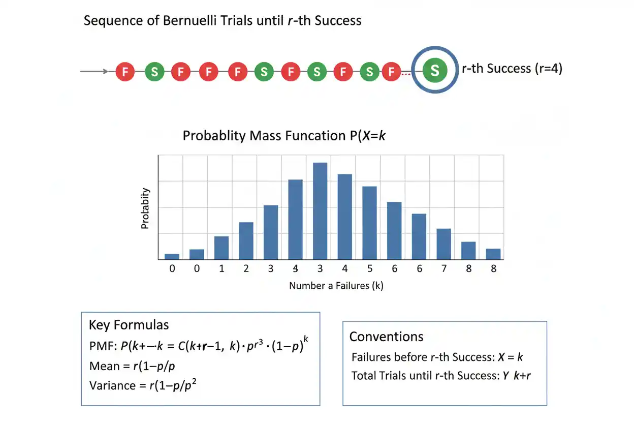
The negative binomial distribution is a discrete probability distribution used to model how many failures occur before a specified number of successes is reached in a sequence of independent Bernoulli trials. Unlike the ordinary binomial distribution, which fixes the total number of trials and counts successes, the negative binomial fixes the required number of successes and allows the number of trials or failures to vary. If K represents the number of failures before the r-th success, the negative binomial probability mass function is P(K = k) = C(k + r − 1, k)p^r(1 − p)^k, where p is the constant probability of success on each independent trial. A second common convention counts the total number of trials required to obtain r successes, so understanding exactly what the random variable counts is essential before applying a formula. Under the failures-before-r-th-success convention, the mean is r(1 − p)/p and the variance is r(1 − p)/p². The negative binomial distribution is right-skewed for many parameter combinations, reduces to the geometric distribution when r = 1, and is widely useful for waiting-time and count processes in which repeated independent trials continue until a target number of successes occurs.
The negative binomial distribution belongs to the discrete probability models within core statistics and the broader Statistics & Probability framework. Its center and dispersion can be understood through the general ideas of mean and variance, but its formulas depend specifically on the repeated-trial structure and the parameter convention being used.
What Is the Negative Binomial Distribution?
The negative binomial distribution models repeated independent Bernoulli trials when the process continues until a predetermined number of successes has occurred.
Each trial must have:
P(success) = p
and:
P(failure) = 1 − p
with:
0 < p ≤ 1
The trials are assumed to be independent, and p remains constant from trial to trial.
Suppose the target is:
r successes
The negative binomial random variable can then be defined in two common ways:
K = number of failures before the r-th success
or:
T = total number of trials required to obtain the r-th success
These definitions describe the same underlying process but produce different supports and means.
They are related by:
T = K + r
because the total number of trials consists of:
failures + r successes
Negative Binomial Formula: Failures Before the r-th Success
Let:
K = number of failures before the r-th success
Then:
K ∈ {0, 1, 2, 3, …}
and the probability mass function is:
P(K = k) = C(k + r − 1, k)p^r(1 − p)^k
for:
k = 0, 1, 2, …
where:
- r = required number of successes
- p = probability of success on each trial
- 1 − p = probability of failure
- k = number of failures before success number r
- C(k + r − 1, k) = number of valid arrangements
The combination term can also be written:
C(k + r − 1, r − 1)
because:
C(n,k) = C(n,n−k)
Thus, an equivalent negative binomial formula is:
P(K = k) = C(k + r − 1, r − 1)p^r(1 − p)^k
Why the Negative Binomial Formula Works
Suppose we want exactly k failures before the r-th success.
The final trial must be a success.
Before that final success, there must be:
r − 1 successes
and:
k failures
distributed among:
k + r − 1
positions.
The number of possible arrangements is therefore:
C(k + r − 1, k)
Each valid sequence contains exactly:
r successes
and:
k failures
so its probability is:
p^r(1 − p)^k
Multiplying the number of valid sequences by the probability of each sequence gives:
P(K = k) = C(k + r − 1, k)p^r(1 − p)^k
The requirement that the last trial be the r-th success is what distinguishes the negative binomial calculation from a fixed-length binomial count.
Negative Binomial Formula: Total Trials Convention
Suppose instead:
T = total number of trials required to obtain r successes
Then:
T ∈ {r, r + 1, r + 2, …}
If:
T = t
the first:
t − 1
trials must contain exactly:
r − 1
successes, and trial t must be the final success.
Therefore:
P(T = t) = C(t − 1, r − 1)p^r(1 − p)^(t − r)
for:
t = r, r + 1, r + 2, …
Because:
K = T − r
the two formulations are equivalent.
For example:
K = 4 failures before the 3rd success
means:
T = 4 + 3 = 7 total trials
to obtain the third success.
Negative Binomial Example
Suppose each independent trial has:
p = 0.40
probability of success.
We continue until:
r = 3
successes occur.
What is the probability of observing exactly:
k = 4
failures before the third success?
Use:
P(K = k) = C(k + r − 1, k)p^r(1 − p)^k
Substitute:
k = 4
r = 3
p = 0.40
Then:
P(K = 4) = C(4 + 3 − 1, 4)(0.40)^3(0.60)^4
P(K = 4) = C(6,4)(0.40)^3(0.60)^4
Since:
C(6,4) = 15
we have:
P(K = 4) = 15(0.064)(0.1296)
P(K = 4) = 0.124416
Therefore:
P(K = 4) ≈ 0.1244
or approximately:
12.44%
There is about a 12.44% probability that four failures occur before the third success.
The Same Example Using Total Trials
Four failures and three successes require:
7 total trials
Therefore:
T = 7
Using the total-trials formula:
P(T = 7) = C(7 − 1, 3 − 1)(0.40)^3(0.60)^(7 − 3)
P(T = 7) = C(6,2)(0.40)^3(0.60)^4
P(T = 7) = 15(0.064)(0.1296)
P(T = 7) = 0.124416
The probability is identical, as expected.
The two statements:
Four failures occur before the third success.
and:
The third success occurs on trial seven.
describe exactly the same event.
What the Combination Term Counts
For the example:
r = 3
k = 4
the final trial must be a success.
The first six trials must therefore contain:
2 successes
and:
4 failures
The number of ways to position the two successes among the first six trials is:
C(6,2)
= 15
Equivalently, choose the four failure positions:
C(6,4)
= 15
Each valid sequence ends with the third success.
One example is:
S, F, F, S, F, F, S
Another is:
F, S, F, F, S, F, S
Both contain four failures before the third success.
Conditions for a Negative Binomial Distribution
A standard negative binomial model requires several structural conditions.
Two Outcomes Per Trial
Each trial must have two relevant outcomes:
success
or:
failure
The labels are mathematical.
A “success” can represent any event being counted, including an equipment failure, customer arrival, or other outcome, provided it is defined consistently.
Independent Trials
The result of one trial should not alter the probability of later outcomes.
If observing a failure changes the probability of success on the next trial, the ordinary negative binomial model may not apply.
Constant Success Probability
Every trial must have the same:
p
If p changes systematically as trials continue, a single negative binomial distribution with fixed p does not exactly describe the process.
Fixed Number of Required Successes
The target:
r
must be specified before the sequence is evaluated.
The random quantity is then the number of failures or total trials required to reach that target.
Negative Binomial PMF
Using the failures-before-success convention:
P(K = k) = C(k + r − 1, k)p^r(1 − p)^k
The possible values are:
k = 0, 1, 2, …
This is a probability mass function because the negative binomial random variable is discrete.
The probabilities satisfy:
P(K = k) ≥ 0
and:
Σ from k=0 to ∞ P(K = k) = 1
The infinite support means there is no fixed maximum number of failures when:
p < 1
A sufficiently long run of failures always has positive probability.
Probability of Zero Failures
Suppose:
K = 0
This means the first r trials are all successes.
Using the formula:
P(K = 0) = C(r − 1, 0)p^r(1 − p)^0
Since:
C(r − 1,0) = 1
and:
(1 − p)^0 = 1
we obtain:
P(K = 0) = p^r
For:
r = 3
and:
p = 0.40
we have:
P(K = 0) = 0.40^3
= 0.064
Therefore, there is a:
6.4%
probability that the first three trials are all successes.
Probability of One Failure Before r Successes
For:
k = 1
the formula becomes:
P(K = 1) = C(r,1)p^r(1 − p)
For:
r = 3
and:
p = 0.40
we have:
P(K = 1) = C(3,1)(0.40)^3(0.60)
= 3(0.064)(0.60)
= 0.1152
Therefore:
P(K = 1) = 11.52%
The single failure can occur in any of the first three positions before the final required success.
Probability of Two Failures
For the same:
r = 3
and:
p = 0.40
calculate:
P(K = 2)
Using:
P(K = 2) = C(4,2)(0.40)^3(0.60)^2
Since:
C(4,2) = 6
we obtain:
P(K = 2) = 6(0.064)(0.36)
P(K = 2) = 0.13824
Therefore:
P(K = 2) ≈ 13.82%
Negative Binomial Cumulative Probability
The cumulative distribution function is:
P(K ≤ k)
It can be calculated by summing the PMF:
P(K ≤ k) = Σ from j=0 to k C(j + r − 1,j)p^r(1 − p)^j
For small k, direct summation is straightforward.
For larger calculations, statistical software typically evaluates the cumulative probability directly.
CDF Example
Using:
r = 3
p = 0.40
what is the probability of at most two failures before the third success?
We want:
P(K ≤ 2)
Therefore:
P(K ≤ 2) = P(K=0) + P(K=1) + P(K=2)
From the previous calculations:
P(K=0) = 0.064
P(K=1) = 0.1152
P(K=2) = 0.13824
Thus:
P(K ≤ 2) = 0.064 + 0.1152 + 0.13824
P(K ≤ 2) = 0.31744
Therefore:
P(K ≤ 2) ≈ 31.74%
Probability of More Than Two Failures
Use the complement:
P(K > 2) = 1 − P(K ≤ 2)
Therefore:
P(K > 2) = 1 − 0.31744
P(K > 2) = 0.68256
So there is approximately a:
68.26%
probability that more than two failures occur before the third success.
Complement calculations are often easier than adding a long upper tail directly.
Probability Over a Range
Suppose we need:
P(a ≤ K ≤ b)
This can be calculated as:
P(K ≤ b) − P(K ≤ a − 1)
Alternatively, sum the individual negative binomial probabilities:
Σ from k=a to b P(K=k)
For discrete distributions, careful attention to endpoints matters.
For example:
P(2 ≤ K ≤ 5)
includes:
K = 2, 3, 4, 5
and excludes:
K = 1
and:
K = 6
Mean of the Negative Binomial Distribution
Under the failures-before-r-th-success convention:
E(K) = r(1 − p)/p
This gives the expected number of failures before r successes occur.
For:
r = 3
p = 0.40
the expected number of failures is:
E(K) = 3(0.60)/0.40
E(K) = 1.8/0.40
E(K) = 4.5
Therefore, the long-run average number of failures before the third success is:
4.5
The expected value does not have to be an integer even though K can take only integer values.
Mean Under the Total-Trials Convention
Since:
T = K + r
we have:
E(T) = E(K) + r
Therefore:
E(T) = r(1 − p)/p + r
Factor r:
E(T) = r[(1 − p)/p + 1]
E(T) = r/p
Thus:
E(T) = r/p
For:
r = 3
and:
p = 0.40
we obtain:
E(T) = 3/0.40
E(T) = 7.5
So an average of:
7.5 total trials
is required to obtain three successes.
Again, a theoretical mean can be non-integer even when the variable itself takes only integers.
Variance of the Negative Binomial Distribution
Under either convention:
Var = r(1 − p)/p²
because adding the constant r to convert failures into total trials does not change variance.
For:
r = 3
and:
p = 0.40
we have:
Var(K) = 3(0.60)/(0.40)²
= 1.8/0.16
= 11.25
Therefore:
Variance = 11.25
The corresponding standard deviation is:
SD = √11.25
SD ≈ 3.354
The waiting process therefore has considerable variability around its mean.
Mean and Variance Compared
For the failures convention:
Mean = r(1 − p)/p
and:
Variance = r(1 − p)/p²
Dividing variance by the mean gives:
Var(K)/E(K) = 1/p
when the mean is nonzero.
Since:
0 < p ≤ 1
we have:
1/p ≥ 1
Therefore, for 0 < p < 1:
Variance > Mean
under the failures-count convention.
This mean–variance relationship is one reason the negative binomial family is useful in count modeling when observed variability exceeds what a Poisson mean–variance equality would allow.
Standard Deviation
The standard deviation is:
SD = √[r(1 − p)]/p
because:
Var = r(1 − p)/p²
and:
p > 0
For:
r = 3
p = 0.40
we obtain:
SD = √1.8/0.40
≈ 3.354
Unlike variance, standard deviation is measured in the same units as the count variable.
Here, those units are:
number of failures
or:
number of trials
depending on the convention.
Negative Binomial as a Sum of Geometric Waiting Times
The negative binomial distribution can be understood as the sum of independent geometric waiting components.
Suppose:
G₁, G₂, …, Gᵣ
represent the numbers of failures encountered before successive successes.
Each:
Gᵢ
has a geometric failures-before-success distribution with:
E(Gᵢ) = (1 − p)/p
and:
Var(Gᵢ) = (1 − p)/p²
Then:
K = G₁ + G₂ + … + Gᵣ
Therefore:
E(K) = r(1 − p)/p
and, under independence:
Var(K) = r(1 − p)/p²
This provides an intuitive derivation of the negative binomial mean and variance.
Negative Binomial and Geometric Distribution
When:
r = 1
the negative binomial PMF becomes:
P(K = k) = C(k,k)p(1 − p)^k
Since:
C(k,k) = 1
we get:
P(K = k) = p(1 − p)^k
This is the geometric distribution under the convention that counts failures before the first success.
Thus:
Geometric distribution = negative binomial with r = 1
The negative binomial generalizes the geometric waiting-time idea from the first success to the r-th success.
Negative Binomial vs Binomial Distribution
The two distributions use repeated Bernoulli trials but reverse what is fixed and what is random.
Binomial Distribution
Fix:
n = number of trials
Count:
X = number of successes
The support is:
0, 1, …, n
Negative Binomial Distribution
Fix:
r = required number of successes
Count either:
K = failures before the r-th success
or:
T = total trials until the r-th success
The upper support is unbounded when:
p < 1
The key contrast is:
Binomial → fixed number of trials
Negative binomial → fixed number of successes
Example: Binomial vs Negative Binomial
Suppose:
p = 0.40
Question A asks:
What is the probability of exactly three successes in seven trials?
That is a binomial question.
Question B asks:
What is the probability that the third success occurs on trial seven?
That is a negative binomial question.
For Question B, trial seven must be a success and the first six trials must contain exactly two successes.
Therefore:
P(T = 7) = C(6,2)(0.40)^3(0.60)^4
The fixed stopping condition makes the structure different from simply counting three successes anywhere among seven trials.
Why the Final Trial Matters
For total trials:
T = t
the t-th trial must be the r-th success.
If we used:
C(t,r)
instead of:
C(t−1,r−1)
we would count arrangements where the r-th success occurred before trial t.
Those sequences would have already stopped.
Therefore, the valid arrangements involve only the first:
t − 1
positions, containing:
r − 1
successes.
The final position is fixed as success.
That is why:
C(t−1,r−1)
appears in the total-trials PMF.
Negative Binomial and Success Odds
The success probability p can also be expressed through odds.
Success odds in favor are:
p/(1 − p)
while failure-to-success odds are:
(1 − p)/p
For:
p = 0.40
the odds in favor of success are:
0.40/0.60
= 2/3
Understanding the distinction between probability and odds formats is useful because the two quantities describe the same event likelihood using different numerical scales.
The negative binomial PMF itself should still be evaluated using probabilities p and 1 − p unless a parameterization explicitly defines otherwise.
Effect of Increasing p
For fixed r, increasing p causes successes to occur more quickly on average.
The expected failures are:
E(K) = r(1 − p)/p
Suppose:
r = 5
If:
p = 0.25
then:
E(K) = 5(0.75)/0.25
= 15
If:
p = 0.50
then:
E(K) = 5(0.50)/0.50
= 5
If:
p = 0.80
then:
E(K) = 5(0.20)/0.80
= 1.25
Larger success probability produces shorter expected waits.
Effect of Increasing r
For fixed p, increasing the required number of successes increases both the expected waiting count and its variance.
Because:
E(K) = r(1 − p)/p
the mean grows linearly with r.
Likewise:
Var(K) = r(1 − p)/p²
also grows linearly with r.
If the target number of successes doubles, both the expected failures and variance double.
The standard deviation increases only by the square root of that factor because:
SD ∝ √r
Shape of the Negative Binomial Distribution
The negative binomial distribution is often right-skewed, particularly when:
- r is small,
- p is small,
- long waits before the required successes are plausible.
As r grows, the distribution can become less strongly skewed.
The exact shape depends jointly on:
r
and:
p
Unlike a symmetric normal distribution, a negative binomial variable cannot take arbitrary negative values and often has a substantial right tail.
Therefore, a normal approximation should be used only when justified by the parameters and analytical purpose.
Mode of the Negative Binomial Distribution
For failures K before r successes, when:
r > 1
a mode is given by:
floor[(r − 1)(1 − p)/p]
with a possible adjacent tie when the unrounded quantity is an integer.
For:
r = 3
and:
p = 0.40
calculate:
(r − 1)(1 − p)/p
= 2(0.60)/0.40
= 3
In this boundary case, adjacent values can share the maximum probability under the usual negative binomial PMF.
For many practical calculations, directly evaluating nearby PMF values is a reliable way to confirm the modal count.
The mode should not be confused with the mean, particularly in a skewed distribution.
Mean, Median, and Mode Need Not Coincide
For a skewed negative binomial distribution:
- the mean,
- median,
- mode
can differ substantially.
This is why the broader distinction among mean, median, mode matters when summarizing observed waiting counts.
The theoretical mean has a simple exact formula.
The median generally does not have an equally simple universal closed-form expression.
The mode depends on r and p and may involve a tie.
A single center should therefore not be assumed to characterize the entire distribution.
Mean Absolute Deviation of Negative Binomial Data
Observed negative binomial counts can be summarized descriptively using statistics beyond theoretical variance.
For example, the mean absolute deviation can describe the average absolute distance of observed counts from their sample mean.
However, sample mean absolute deviation and theoretical negative binomial variance answer different questions.
The theoretical variance:
r(1 − p)/p²
comes directly from the probability model.
A sample absolute-deviation statistic summarizes the particular observed data.
One should not substitute for the other without understanding the purpose of the analysis.
Negative Binomial and Overdispersion
In count-data modeling, one reason the negative binomial family is important is its ability to represent variance larger than the mean.
A basic Poisson model imposes:
Var(X) = E(X)
The negative binomial family can allow:
Var(X) > E(X)
under common count parameterizations.
This additional dispersion can better describe count data with greater heterogeneity than the Poisson model permits.
However, observing sample variance greater than the sample mean does not automatically prove that a negative binomial model is correct.
Other sources of extra variation include:
- omitted heterogeneity,
- clustering,
- zero inflation,
- dependence,
- changing exposure,
- model misspecification.
Distribution selection requires more than comparing two summary statistics.
Alternative Negative Binomial Parameterizations
The negative binomial distribution is notorious for inconsistent notation across textbooks and software.
One source may define:
X = failures before r successes
Another may define:
X = total trials until r successes
A third may reverse the role of success and failure probabilities.
Some statistical software parameterizes the distribution using:
- a mean μ,
- a size or shape parameter,
- a dispersion parameter,
rather than r and p directly.
Therefore, before applying a formula, always identify:
- What does the random variable count?
- What does p represent?
- What is the support?
- What parameterization does the software use?
Failing to answer these questions can produce correct arithmetic for the wrong distribution.
Conversion Between Failures and Total Trials
If:
K = failures before r successes
and:
T = total trials until r successes
then:
T = K + r
Therefore:
K = T − r
Their expected values satisfy:
E(T) = E(K) + r
Their variances satisfy:
Var(T) = Var(K)
because adding a constant does not change variance.
Their probabilities map directly:
P(T = t) = P(K = t − r)
for:
t ≥ r
This conversion makes it easy to translate between the two conventions.
Boundary Case p = 1
If:
p = 1
every trial succeeds.
Therefore, no failures occur before r successes:
K = 0
with probability:
1
The total number of trials is:
T = r
with probability:
1
For the failures convention:
E(K) = r(1 − 1)/1 = 0
and:
Var(K) = 0
The distribution becomes degenerate rather than random.
What Happens as p Approaches Zero?
As:
p → 0⁺
success becomes extremely rare.
The expected number of failures:
E(K) = r(1 − p)/p
grows without bound.
Likewise:
Var(K) = r(1 − p)/p²
becomes extremely large.
Therefore, the negative binomial waiting-time distribution develops a very long right tail when the per-trial success probability is very small.
The value:
p = 0
is excluded because the required successes would never occur.
Independence Is Essential
Suppose each failure makes a future success more likely.
Then:
p
changes conditionally after each outcome.
The standard negative binomial formula:
C(k+r−1,k)p^r(1−p)^k
no longer describes the exact probability structure.
Similarly, repeated observations from the same system may be correlated because of learning, fatigue, changing environment, or resource depletion.
A sequence can look superficially like repeated binary trials without satisfying the independence assumption.
The data-generating process must be considered.
Constant p Is Essential
Imagine repeated attempts where skill improves after each failure.
Then:
p₁ < p₂ < p₃ < …
The success probability is no longer constant.
The probability of a particular sequence depends on the individual trial-specific probabilities rather than one common p.
Likewise, sampling without replacement from a finite population changes the composition after each draw and generally changes the success probability.
In such settings, an ordinary negative binomial model may be inappropriate.
Negative Binomial and Sampling Without Replacement
The standard negative binomial distribution assumes repeated independent trials with replacement-like probability stability.
Suppose a finite container contains successful and unsuccessful objects and items are removed after each draw.
After each removal, the proportion of successful objects can change.
Therefore:
P(success on next draw)
depends on previous outcomes.
The resulting waiting-time process is generally not negative binomial.
A large population with only a tiny fraction sampled may sometimes make the independent approximation reasonable, but that approximation should be justified.
Negative Binomial vs Normal Distribution
The negative binomial is discrete and generally asymmetric.
The normal distribution is continuous and symmetric.
For some parameter combinations, particularly when the relevant expected count is large and skewness is modest, a normal approximation can sometimes be useful.
A rough approximation would match:
Mean = r(1 − p)/p
and:
Variance = r(1 − p)/p²
under the failures convention.
However, the normal distribution permits negative values, while a failure count cannot be negative.
Continuity corrections and tail accuracy also matter.
Exact negative binomial probabilities are generally preferable when they are computationally available.
Negative Binomial Skewness
For the failures-before-r-successes convention, skewness is positive for ordinary nondegenerate parameter values.
A common expression is:
Skewness = (2 − p)/√[r(1 − p)]
The value is positive because:
0 < p < 1
implies:
2 − p > 0
As r increases, the denominator increases, so skewness generally decreases.
This helps explain why larger-r negative binomial distributions can appear more nearly symmetric.
Probability Generating Function
For K counting failures before r successes, the probability generating function is:
G(s) = [p / (1 − (1 − p)s)]^r
for values of s where the expression is defined.
This compact function can be used to derive moments.
For example:
G'(1) = E(K)
which yields:
r(1 − p)/p
Higher derivatives can help derive additional properties.
The probability generating function is especially useful in theoretical work with discrete random variables.
Moment Generating Function
The moment generating function for the failures convention is:
M(t) = [p / (1 − (1 − p)e^t)]^r
for t values satisfying the convergence condition.
Differentiating at:
t = 0
produces the moments.
In particular:
M'(0) = E(K)
and the second derivative contributes to:
Var(K)
These formulas are useful theoretically, although routine probability calculations usually need only the PMF, CDF, mean, and variance.
Negative Binomial Additivity
An important property is that independent negative binomial variables with the same success probability can add naturally.
Suppose:
K₁ ~ NB(r₁,p)
and:
K₂ ~ NB(r₂,p)
independently under the failures convention.
Then:
K₁ + K₂ ~ NB(r₁ + r₂,p)
This follows naturally from the waiting-time interpretation.
Waiting for r₁ successes and then another r₂ successes is equivalent to waiting for:
r₁ + r₂
successes in total when the same independent-trial probability p continues.
Estimating p When r Is Known
Suppose observations:
k₁, k₂, …, kₙ
are independent negative binomial failure counts with known r.
The theoretical mean is:
E(K) = r(1 − p)/p
Set the sample mean approximately equal to the model mean:
k̄ = r(1 − p)/p
Solve for p.
Multiply by p:
pk̄ = r(1 − p)
pk̄ = r − rp
Collect p terms:
p(k̄ + r) = r
Therefore:
p̂ = r/(r + k̄)
This estimator also arises from maximum likelihood under the standard failures-count model when r is known.
Estimation Example
Suppose:
r = 3
and the observed average number of failures is:
k̄ = 4.5
Then:
p̂ = 3/(3 + 4.5)
p̂ = 3/7.5
p̂ = 0.40
This matches the parameter used in the earlier example.
The estimate is still subject to sampling uncertainty.
A single fitted value of p should not be treated as though the population probability were known exactly.
Negative Binomial Regression
The term negative binomial regression refers to a regression framework for overdispersed count outcomes.
It is related to the negative binomial probability family but is not the same task as calculating a waiting-time PMF.
In regression applications, the mean count may be modeled through predictors, often using a logarithmic link:
log(μᵢ) = β₀ + β₁xᵢ + …
The distribution may be parameterized in terms of:
μ
and a dispersion or size parameter rather than directly through the waiting-time p convention.
Therefore, formulas from one parameterization should not be inserted into another without conversion.
Negative Binomial vs Ordinary Regression Models
A negative binomial count outcome is discrete and nonnegative.
Ordinary least-squares regression assumes a different mean-error structure and can produce predictions inconsistent with count behavior.
Specialized count regression can better accommodate:
- integer outcomes,
- skewness,
- variance linked to the mean,
- overdispersion.
The choice of regression family should follow the response variable and data-generating process rather than being based only on whether a fitted curve looks visually reasonable.
Negative Binomial and Statistical Inference
When r or p must be estimated from sample data, parameter estimates have sampling uncertainty.
Inference can include:
- standard errors,
- confidence intervals,
- likelihood-based tests,
- model comparisons.
A small p-value in a fitted model does not mean there is a small probability that the null hypothesis is true.
Likewise, a confidence interval should be interpreted through its repeated-sampling coverage rather than as an automatic posterior probability statement about a fixed parameter.
The inferential method must match the parameterization and sampling structure.
Negative Binomial and Practical Interpretation
Suppose a fitted negative binomial model estimates:
p = 0.80
with:
r = 5
The expected failures are:
E(K) = 5(0.20)/0.80
= 1.25
Suppose another process has:
p = 0.20
with the same r.
Then:
E(K) = 5(0.80)/0.20
= 20
The second process requires dramatically more failures on average before five successes occur.
This direct waiting-time interpretation can be more informative than reporting model parameters without context.
Common Negative Binomial Mistakes
One of the most common mistakes is failing to identify the random-variable convention.
The formulas for:
failures before r successes
and:
total trials until r successes
have different support and means.
Another mistake is using:
C(k+r,k)
instead of:
C(k+r−1,k)
for the failures-count PMF.
The final trial must be the r-th success, which reduces the freely arranged positions by one.
A third error is confusing the negative binomial with the ordinary binomial distribution.
Binomial fixes the total trial count; negative binomial fixes the target number of successes.
Another mistake is forgetting the combination term. Unlike a geometric distribution with r = 1, multiple arrangements can lead to the same negative binomial failure count.
Analysts can also reverse p and 1 − p because some software packages define parameters differently.
Another common error is applying the model when success probability changes or trials are dependent.
Finally, a theoretical mean such as 4.5 failures should not be interpreted as requiring a half failure in an actual sequence. Expected values are long-run averages and need not belong to the support.
How to Solve a Negative Binomial Problem
A reliable approach is:
Step 1: Identify Success and Failure
Define exactly what constitutes:
success
and:
failure
Step 2: Identify p
Determine:
p = P(success)
Then:
1 − p = P(failure)
Step 3: Identify r
Find the required number of successes.
Step 4: Determine What the Random Variable Counts
Does it count:
failures before the r-th success
or:
total trials until the r-th success?
This determines the formula and support.
Step 5: Translate the Question
Examples include:
Exactly k failures → P(K = k)
At most k failures → P(K ≤ k)
More than k failures → P(K > k)
r-th success on trial t → P(T = t)
Step 6: Apply the Formula
Failures convention:
P(K = k) = C(k+r−1,k)p^r(1−p)^k
Total trials:
P(T = t) = C(t−1,r−1)p^r(1−p)^(t−r)
Step 7: Check the Support
Make sure:
k ≥ 0
or:
t ≥ r
Step 8: Interpret the Result
State the probability in terms of the actual stopping event.
Worked Example: Fifth Success on Trial 12
Suppose:
p = 0.30
and we want the probability that the fifth success occurs on trial:
t = 12
Then:
r = 5
There must be:
4 successes
among the first:
11 trials
and trial 12 must be success number five.
The number of failures is:
12 − 5 = 7
Therefore:
P(T = 12) = C(11,4)(0.30)^5(0.70)^7
Since:
C(11,4) = 330
the probability is:
P(T = 12) = 330(0.30)^5(0.70)^7
This expression can then be evaluated numerically.
The structural setup is the crucial part: the final trial must be the fifth success.
Worked Example: At Most Two Failures Before the Third Success
Let:
r = 3
p = 0.40
We want:
P(K ≤ 2)
Calculate:
P(K=0) = 0.064
P(K=1) = 0.1152
P(K=2) = 0.13824
Therefore:
P(K ≤ 2) = 0.31744
Thus, there is approximately a:
31.74%
chance that the third success occurs after no more than two failures.
Equivalently, the third success occurs within the first:
5 trials
because:
3 successes + 2 failures = 5 trials
Worked Example: Expected Trials
Suppose:
r = 8
and:
p = 0.50
The expected total number of trials is:
E(T) = r/p
E(T) = 8/0.50
E(T) = 16
Expected failures are:
E(K) = r(1 − p)/p
= 8(0.50)/0.50
= 8
Therefore, on average:
8 failures + 8 successes = 16 total trials
are required.
How to Report a Negative Binomial Result
A probability calculation should identify the parameterization.
For example:
Let K denote the number of failures before the third success, with independent trials and p = 0.40. Then P(K = 4) = 0.1244.
A direct interpretation is:
There is approximately a 12.44% probability of observing four failures before the third success.
If using total trials instead:
Let T denote the number of trials required to obtain three successes. Then P(T = 7) = 0.1244.
Both statements are correct because:
T = K + 3
Stating the convention prevents ambiguity.
Frequently Asked Questions About the Negative Binomial
What is the negative binomial distribution?
The negative binomial distribution models repeated independent Bernoulli trials until a specified number of successes has occurred.
What does the negative binomial count?
Under one common convention, it counts failures before the r-th success. Under another, it counts total trials required for the r-th success.
What is the negative binomial formula?
For failures K before r successes:
P(K = k) = C(k+r−1,k)p^r(1−p)^k
What is the total-trials formula?
If T counts total trials until the r-th success:
P(T = t) = C(t−1,r−1)p^r(1−p)^(t−r)
for:
t = r, r+1, …
What is the support of the negative binomial distribution?
For failures before r successes:
K = 0, 1, 2, …
For total trials until r successes:
T = r, r+1, r+2, …
What does p represent?
p is the constant probability of success on each independent trial.
What does r represent?
r is the predetermined number of successes required before the process stops.
What is the mean of the negative binomial distribution?
If K counts failures:
E(K) = r(1−p)/p
If T counts total trials:
E(T) = r/p
What is the variance?
Under either shifted convention:
Var = r(1−p)/p²
Why is the variance the same under both conventions?
Because:
T = K + r
and adding a constant does not change variance.
What is the difference between negative binomial and binomial distributions?
Binomial fixes the number of trials and counts successes. Negative binomial fixes the number of required successes and counts failures or total trials until that target is reached.
What is the difference between negative binomial and geometric distributions?
The geometric distribution stops at the first success. The negative binomial stops at the r-th success. Geometric is the special case:
r = 1
Why does the formula use C(k+r−1,k)?
Before the final required success, k failures and r−1 successes can appear in any order. The combination counts those valid arrangements.
Why must the final trial be a success?
The process stops exactly when the r-th success occurs, so the last trial in the counted sequence must be success number r.
Can the negative binomial random variable be zero?
Under the failures convention, yes:
K = 0
means the first r trials are all successes.
Under the total-trials convention, the smallest possible value is:
T = r
Can the negative binomial distribution have an infinite number of possible values?
Yes, when p < 1. There is no fixed maximum number of failures or total trials before the required successes occur.
What happens when p = 1?
Every trial succeeds. Therefore:
K = 0
and:
T = r
with probability one.
Can p equal zero?
Not in an ordinary finite waiting-time negative binomial model. If p = 0, the required successes never occur.
Are negative binomial trials independent?
Yes, independence is a defining assumption of the standard repeated-trial version.
Can the success probability change between trials?
Not under the basic negative binomial model. A changing success probability requires another probability structure.
Is the negative binomial distribution discrete?
Yes. It assigns probabilities to integer counts.
Is the negative binomial distribution usually skewed?
It is commonly right-skewed, especially when success probability or the required number of successes is small. Its shape depends on r and p.
Can the negative binomial distribution approximate a normal distribution?
For some parameter combinations, particularly when counts are sufficiently large and skewness is modest, a normal approximation may be useful. Exact probabilities are preferable when readily available.
Why is the negative binomial useful for overdispersed counts?
Under common count parameterizations, it can allow variance to exceed the mean, providing more flexibility than a Poisson model.
Does variance greater than the mean prove the data are negative binomial?
No. Overdispersion can have many causes, and model selection requires examining the full probability structure.
What is negative binomial regression?
Negative binomial regression is a regression model for count responses using a negative binomial probability family. Its parameterization is often expressed in terms of a mean and dispersion parameter rather than the simple waiting-time r and p notation.
How do I know which negative binomial formula software uses?
Check the software definition for the random variable, support, probability parameter, and size or dispersion parameter. Negative binomial parameterization varies substantially across systems.
Does the negative binomial mean have to be an integer?
No. Expected values are long-run averages and can be non-integer even though observed counts are integers.




