Poisson Distribution: Definition, Formula & Example

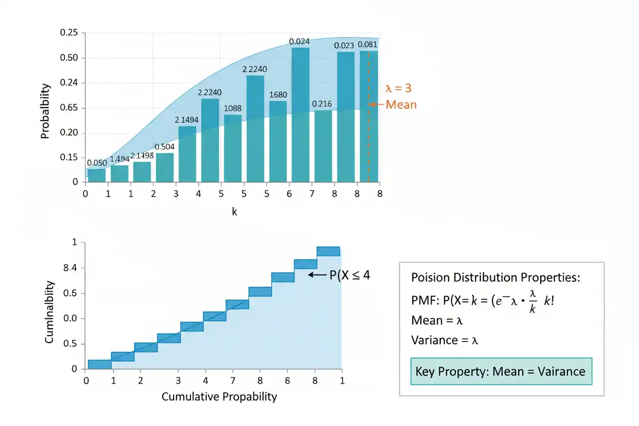
The Poisson distribution is a discrete probability distribution used to model the number of events occurring within a fixed interval of time, space, area, volume, or another exposure unit when events occur independently at an approximately constant average rate. Its single parameter, λ, represents the expected number of events in the specified interval, and the probability of observing exactly k events is calculated with P(X = k) = e^−λ λ^k/k!. A distinctive property of the Poisson distribution is that its theoretical mean and variance are both equal to λ, so the same parameter determines both the center and the spread of the count model. The distribution includes only nonnegative integer values, can be strongly right-skewed when λ is small, and becomes progressively more symmetric as λ increases. It is particularly useful for random counts such as arrivals, defects, incidents, or occurrences when the underlying assumptions are reasonable, but it can fit poorly when events cluster, inhibit one another, rates change substantially, or observed variability differs materially from the Poisson mean–variance relationship. Correct use therefore requires more than applying the probability formula: the event definition, exposure interval, rate stability, dependence structure, and empirical dispersion all need to support the model.

The Poisson distribution is one of the fundamental discrete models within core statistics and the broader Statistics & Probability framework. Its probabilities build directly on the general rules of probability, while cumulative probabilities can also be interpreted through discrete percentiles when count thresholds are the quantity of interest.

What Is the Poisson Distribution?

The Poisson distribution models a count:

X = number of events in a specified interval

where the possible values are:

X = 0, 1, 2, 3, …

If X follows a Poisson distribution with mean rate λ, the notation is:

X ~ Poisson(λ)

where:

λ > 0

The parameter λ represents the expected number of events in the interval being modeled. If a location receives an average of four independent arrivals per hour under a stable-rate Poisson model, then:

λ = 4

for a one-hour interval.

If the same constant-rate model is applied to a two-hour interval, the expected count becomes:

λ = 8

provided the rate remains constant and the exposure doubles.

The interval therefore matters as much as the numerical rate.

Poisson Distribution Formula

The probability mass function is:

P(X = k) = e^−λ λ^k/k!

for:

k = 0, 1, 2, …

where:

• X = event count
• k = specified nonnegative integer count
• λ = expected number of events in the interval
• e ≈ 2.71828
• k! = factorial of k

The factorial is:

k! = k(k − 1)(k − 2)…(2)(1)

with:

0! = 1

The Poisson distribution is discrete, so its probability function assigns positive probability to individual integer counts.

That distinguishes it from a continuous distribution, where the probability at one exact point is zero.

Poisson Distribution Example

Suppose a system receives an average of:

λ = 4

events per hour, and a Poisson model is appropriate.

What is the probability of observing exactly:

k = 3

events in the next hour?

Use:

P(X = k) = e^−λ λ^k/k!

Substitute:

P(X = 3) = e^−4 4³/3!

Now:

4³ = 64

and:

3! = 6

Therefore:

P(X = 3) = e^−4(64/6)

Since:

e^−4 ≈ 0.0183156

we obtain:

P(X = 3) ≈ 0.19537

Therefore:

P(X = 3) ≈ 19.54%

Under the model, there is approximately a 19.54% probability of observing exactly three events in the one-hour interval.

Why the Poisson Formula Works

The Poisson formula combines three mathematical components:

e^−λ

λ^k

1/k!

The term:

λ^k

reflects the expected event rate raised according to the count being considered, while:

k!

adjusts for the combinatorial ordering of indistinguishable events. The normalization term:

e^−λ

ensures that the total probability across all nonnegative integer counts equals one.

Therefore:

Σ from k=0 to ∞ P(X = k) = 1

The formula is not an arbitrary curve fitted to counts. It arises naturally from a limiting model for many independent opportunities for rare events and from the assumptions of a homogeneous Poisson process.

Probability of Zero Events

Set:

k = 0

in the Poisson formula:

P(X = 0) = e^−λ λ⁰/0!

Since:

λ⁰ = 1

and:

0! = 1

we obtain:

P(X = 0) = e^−λ

For:

λ = 4

this becomes:

P(X = 0) = e^−4

P(X = 0) ≈ 0.01832

Therefore, the probability of no events in an interval with expected count four is approximately:

1.83%

This simple expression is especially useful when calculating the probability of at least one event.

Probability of At Least One Event

Use the complement:

P(X ≥ 1) = 1 − P(X = 0)

Because:

P(X = 0) = e^−λ

we obtain:

P(X ≥ 1) = 1 − e^−λ

For:

λ = 4

the result is:

P(X ≥ 1) = 1 − e^−4

≈ 1 − 0.01832

≈ 0.98168

Therefore:

P(X ≥ 1) ≈ 98.17%

The complement is considerably easier than adding the probabilities of 1, 2, 3, and every larger count.

Probability of Exactly One Event

For:

k = 1

the formula becomes:

P(X = 1) = e^−λ λ

For:

λ = 4

we have:

P(X = 1) = 4e^−4

≈ 0.07326

Therefore:

P(X = 1) ≈ 7.33%

The relationship between adjacent Poisson probabilities also provides an efficient way to calculate this value and subsequent counts without repeatedly evaluating factorials and powers.

Recurrence Formula

Poisson probabilities satisfy:

P(X = k + 1) = P(X = k) × λ/(k + 1)

This relationship follows directly from the PMF.

Starting with:

P(X = 0) = e^−λ

we can calculate successive probabilities.

For:

λ = 4

we have:

P(X = 0) ≈ 0.01832

Then:

P(X = 1) = 0.01832 × 4/1

≈ 0.07326

Next:

P(X = 2) = 0.07326 × 4/2

≈ 0.14653

Then:

P(X = 3) = 0.14653 × 4/3

≈ 0.19537

This recurrence is computationally efficient and makes the changing shape of the distribution easier to understand.

Cumulative Poisson Probability

The cumulative distribution function gives:

P(X ≤ k)

For a Poisson variable:

P(X ≤ k) = Σ from j=0 to k e^−λ λ^j/j!

There is no need to invent a new probability formula for each cumulative question. The CDF is simply the sum of the individual probability masses from zero through the specified count.

For example:

P(X ≤ 2)

equals:

P(X=0) + P(X=1) + P(X=2)

CDF Example

Let:

X ~ Poisson(4)

Find:

P(X ≤ 2)

The required probabilities are approximately:

P(X=0) = 0.01832

P(X=1) = 0.07326

P(X=2) = 0.14653

Therefore:

P(X ≤ 2) ≈ 0.01832 + 0.07326 + 0.14653

P(X ≤ 2) ≈ 0.23810

Thus:

P(X ≤ 2) ≈ 23.81%

Under the model, approximately 23.81% of intervals contain two or fewer events.

Probability of More Than k Events

Use the complement:

P(X > k) = 1 − P(X ≤ k)

For:

X ~ Poisson(4)

and:

k = 2

we found:

P(X ≤ 2) ≈ 0.23810

Therefore:

P(X > 2) ≈ 1 − 0.23810

P(X > 2) ≈ 0.76190

Thus, approximately:

76.19%

of intervals contain more than two events.

Complement calculations are especially useful when the direct upper tail would require summing infinitely many terms.

Probability Over an Interval of Counts

For discrete counts:

P(a ≤ X ≤ b)

can be calculated as:

P(X ≤ b) − P(X ≤ a − 1)

For example:

P(3 ≤ X ≤ 6)

equals:

P(X ≤ 6) − P(X ≤ 2)

Alternatively, add:

P(X=3) + P(X=4) + P(X=5) + P(X=6)

Both methods are equivalent.

The cumulative approach is usually more convenient when software or a CDF table is available.

Mean of the Poisson Distribution

If:

X ~ Poisson(λ)

then:

E(X) = λ

This is one of the defining properties of the model.

For:

X ~ Poisson(4)

the mean count is:

E(X) = 4

That does not mean every interval contains exactly four events.

It means that across many comparable intervals generated by the model, the average count approaches four.

The expected value can also be noninteger.

For example:

λ = 2.7

is a valid Poisson mean even though an observed count can never equal 2.7.

Variance of the Poisson Distribution

The Poisson variance is:

Var(X) = λ

Therefore:

Mean = Variance = λ

For:

X ~ Poisson(4)

we have:

E(X) = 4

and:

Var(X) = 4

The standard deviation is:

SD(X) = √λ

so:

SD(X) = √4

SD(X) = 2

This mean–variance equality is a central structural feature of the Poisson distribution and an important diagnostic when deciding whether the model is plausible for observed count data.

Standard Deviation

For:

X ~ Poisson(λ)

the standard deviation is:

σ = √λ

Suppose:

λ = 25

Then:

Variance = 25

and:

Standard deviation = 5

As λ increases, the absolute spread grows.

However, relative variability decreases because:

SD/Mean = √λ/λ

= 1/√λ

Thus, high-rate Poisson counts are more concentrated around their mean in proportional terms than low-rate counts.

Coefficient of Variation

For a Poisson variable:

CV = SD/Mean

Therefore:

CV = √λ/λ

CV = 1/√λ

For:

λ = 4

we have:

CV = 1/2

= 0.50

For:

λ = 100

we obtain:

CV = 1/10

= 0.10

The distribution becomes less variable relative to its mean as λ grows.

This contributes to its increasingly symmetric appearance at larger rates.

Shape of the Poisson Distribution

The shape depends entirely on λ.

When λ is small, the Poisson distribution is strongly right-skewed because counts cannot fall below zero but can extend arbitrarily far upward.

As λ increases, the center moves right and the distribution becomes increasingly symmetric.

For example:

λ = 0.5

produces a distribution concentrated heavily at zero and one.

By contrast:

λ = 30

produces a broadly bell-shaped discrete pattern centered around 30.

The distribution remains discrete regardless of how large λ becomes.

Skewness

The theoretical skewness of a Poisson distribution is:

Skewness = 1/√λ

For:

λ = 1

skewness is:

1

For:

λ = 4

skewness is:

0.5

For:

λ = 100

skewness is:

0.1

Therefore, right skew decreases as λ increases.

The distribution approaches a more symmetric form but does not literally become a continuous normal distribution.

Kurtosis

The excess kurtosis of a Poisson distribution is:

Excess kurtosis = 1/λ

Therefore, as λ becomes larger:

Excess kurtosis → 0

which is another way the standardized Poisson shape moves toward normal-like behavior.

For:

λ = 4

excess kurtosis is:

0.25

For:

λ = 100

it is:

0.01

These are theoretical population properties rather than statistics calculated from one finite sample.

Mode of the Poisson Distribution

When λ is not an integer, the mode is:

floor(λ)

For example, if:

λ = 4.7

the mode is:

4

When λ is a positive integer, there are two adjacent modes:

λ − 1

and:

λ

For example:

X ~ Poisson(4)

has modes:

3 and 4

The probabilities at those values are equal.

This follows from the recurrence:

P(X=k+1)/P(X=k) = λ/(k+1)

At k = λ − 1, the ratio equals 1 when λ is an integer.

Poisson Distribution Assumptions

A Poisson model is most defensible when its event-count mechanism satisfies an appropriate structure. The exact assumptions are most naturally stated through a homogeneous Poisson process, but the practical ideas can be summarized in terms of independence, stable rate, and event occurrence over a clearly defined exposure.

Events Are Counted Over a Fixed Exposure

The model requires a defined interval such as:

• one hour,
• one kilometer,
• one square meter,
• one production batch,
• one unit of exposure.

Changing that interval generally changes λ.

The Average Rate Is Stable

The expected event rate should remain approximately constant throughout the modeled interval or exposure.

If events become much more frequent at certain times, a single homogeneous Poisson rate may be inappropriate.

Independent Increments

Counts in non-overlapping intervals are independent under a standard Poisson process.

An event occurring in one interval should not directly make another disjoint interval more or less likely to contain events.

Events Do Not Occur in Large Simultaneous Clusters Under the Basic Process

Over a very short interval, the probability of more than one event should become negligible relative to the interval length.

This property leads to individual random event arrivals rather than large instantaneous batches.

Constant Rate Does Not Mean Events Are Evenly Spaced

A Poisson process can have a constant average rate while actual events remain irregular.

Suppose:

λ = 60 per hour

This does not mean one event occurs exactly every minute.

A particular hour might contain:

52 events

another:

67 events

and another:

59 events.

Even within one hour, events can occur close together and then be followed by a long gap.

Constant rate refers to the expected probabilistic structure, not a deterministic schedule.

Changing the Exposure Interval

Suppose a process has rate:

3 events per hour.

For one hour:

λ = 3

For two hours:

λ = 6

For half an hour:

λ = 1.5

provided the rate remains constant.

More generally:

λ = rate × exposure

If the event rate is:

r

per unit exposure and the exposure is:

t

then:

λ = rt

This relationship is central when applying the Poisson distribution across different interval lengths.

Example With a Changed Interval

Suppose an average of:

6 events

occurs every two hours.

The equivalent hourly rate is:

3 events per hour

For a 30-minute interval:

t = 0.5 hours

so:

λ = 3(0.5)

λ = 1.5

The probability of zero events during that half-hour is:

P(X=0) = e^−1.5

≈ 0.2231

Therefore, there is approximately a:

22.31%

chance of observing no events in the half-hour interval under the model.

Poisson Distribution and Probability

The Poisson distribution is one specific application of the broader rules of probability. Its PMF assigns a probability to each possible nonnegative integer count, and those probabilities satisfy the fundamental requirements:

0 ≤ P(X=k) ≤ 1

and:

ΣP(X=k) = 1

Events such as:

X ≥ 5

are formed by combining individual count probabilities.

Complements, unions, and conditional probability concepts still follow the ordinary rules of probability.

The Poisson model supplies the distributional probabilities; it does not replace the general probability framework.

Poisson Percentiles

Because the Poisson distribution is discrete, a percentile is commonly defined as the smallest integer k satisfying:

P(X ≤ k) ≥ q

where q is the desired cumulative probability.

This links the distribution with percentiles, but the discrete nature creates an important difference from smooth continuous distributions.

The CDF jumps at integer counts.

Therefore, there may be no k for which:

P(X ≤ k) = q

exactly.

A percentile can correspond to a cumulative probability somewhat above the requested level.

Discrete Percentile Example

Suppose:

X ~ Poisson(4)

and we want the 90th percentile.

We seek the smallest integer k for which:

P(X ≤ k) ≥ 0.90

For this distribution:

P(X ≤ 6) ≈ 0.8893

while:

P(X ≤ 7) ≈ 0.9489

Therefore, under the common discrete quantile definition:

P90 = 7

because 7 is the first count at which cumulative probability reaches or exceeds 90%.

It is expected that:

P(X ≤ 7)

is larger than exactly 0.90 because the CDF changes in discrete jumps.

Poisson Distribution vs Binomial Distribution

A binomial random variable counts successes in a fixed number of independent Bernoulli trials:

X ~ Binomial(n,p)

A Poisson variable models counts over an exposure interval using a rate parameter:

X ~ Poisson(λ)

The binomial support is finite:

0, 1, …, n

The Poisson support is:

0, 1, 2, …

The models are related through a rare-event limit.

If:

n

is large,

p

is small, and:

np = λ

remains approximately constant, then:

Binomial(n,p)

can be approximated by:

Poisson(λ)

Poisson Approximation to the Binomial

Suppose:

X ~ Binomial(1000, 0.002)

Then:

np = 1000(0.002)

= 2

A Poisson approximation uses:

Y ~ Poisson(2)

The binomial probability of exactly k successes:

C(n,k)p^k(1−p)^(n−k)

can then be approximated by:

e^−2 2^k/k!

The approximation is useful because the Poisson expression can be simpler for rare-event counts.

Its accuracy improves when individual success probabilities are small and the binomial rare-event conditions are suitable.

Why the Poisson Appears as a Rare-Event Limit

Consider a fixed expected number of events λ distributed across n increasingly small independent opportunities.

Set:

p = λ/n

Then:

np = λ

The binomial PMF becomes:

P(X=k) = C(n,k)(λ/n)^k(1−λ/n)^(n−k)

As:

n → ∞

with k fixed, this expression approaches:

e^−λ λ^k/k!

which is the Poisson PMF.

This limiting argument provides a direct mathematical connection between binomial rare events and Poisson counts.

Poisson Distribution vs Negative Binomial

Both models can describe nonnegative count variables, but their mean–variance relationships differ.

For a Poisson distribution:

Mean = Variance = λ

Many negative binomial parameterizations allow:

Variance > Mean

This additional flexibility can make negative binomial models useful when observed counts are substantially more dispersed than a Poisson model predicts.

However, sample variance exceeding the sample mean does not automatically establish that the data are negative binomial.

The cause of extra variation must still be investigated.

Overdispersion

Overdispersion occurs when observed variability is greater than expected under the chosen Poisson model.

A rough descriptive clue is:

Sample variance > Sample mean

by considerably more than would be expected from sampling variability.

Potential causes include:

• heterogeneous event rates,
• clustering,
• dependence,
• omitted predictors,
• excess zeros,
• mixture distributions.

A basic Poisson model forces theoretical variance to equal theoretical mean.

If that restriction is unrealistic, standard errors and probability estimates can be misleading.

Underdispersion

Underdispersion occurs when observed count variability is smaller than a Poisson model would predict.

A rough descriptive pattern is:

Sample variance < Sample mean

Possible causes include:

• regular spacing,
• inhibition between events,
• capacity restrictions,
• strong control mechanisms.

Underdispersion also violates the simple Poisson mean–variance structure.

It should not be ignored simply because overdispersion is more commonly discussed.

Zero Inflation

A Poisson distribution predicts:

P(X=0) = e^−λ

Suppose observed data contain far more zeros than this model expects.

For example, if:

λ = 2

the ordinary Poisson probability of zero is:

e^−2 ≈ 0.1353

If the observed proportion of zero counts is closer to:

50%

the discrepancy may indicate:

• heterogeneous subgroups,
• structural zeros,
• model misspecification,
• zero-inflated processes.

A zero-inflated model is one possible response, but the substantive mechanism should be investigated first.

Estimating λ From Data

Suppose:

X₁, X₂, …, Xₙ

are independent Poisson observations sharing the same λ.

The maximum-likelihood estimator of λ is the sample mean:

λ̂ = x̄

For example, suppose observed counts are:

2, 5, 3, 4, 6

Then:

x̄ = (2 + 5 + 3 + 4 + 6)/5

x̄ = 20/5

x̄ = 4

Therefore:

λ̂ = 4

The fitted Poisson model would use an estimated event count of four per observation interval.

Why the Sample Mean Estimates λ

The Poisson population mean is:

E(X) = λ

Therefore, the arithmetic sample mean is a natural estimator.

The likelihood calculation leads to the same result.

For independent observations x₁,…,xₙ, the likelihood is proportional to:

e^−nλ λ^(Σxᵢ)

after terms not involving λ are separated.

Maximizing its logarithm with respect to λ gives:

λ̂ = Σxᵢ/n

λ̂ = x̄

Thus, the intuitive mean-based estimator and formal maximum-likelihood estimator coincide.

Standard Error of Estimated λ

For independent identically distributed Poisson observations:

Var(X̄) = λ/n

Therefore, the standard error of the sample mean is:

SE(X̄) = √(λ/n)

Since λ is usually unknown, a plug-in estimate is:

SE(λ̂) ≈ √(λ̂/n)

Suppose:

λ̂ = 4

and:

n = 100

Then:

SE ≈ √(4/100)

= √0.04

= 0.2

This quantifies sampling uncertainty around the estimated mean rate under the basic model.

Sums of Independent Poisson Variables

Suppose:

X ~ Poisson(λ₁)

and:

Y ~ Poisson(λ₂)

independently.

Then:

X + Y ~ Poisson(λ₁ + λ₂)

This property extends to any finite collection of independent Poisson variables.

For example:

X ~ Poisson(3)

Y ~ Poisson(5)

independently.

Then:

X + Y ~ Poisson(8)

The expected values add:

3 + 5 = 8

and the variances also add:

3 + 5 = 8

because the variables are independent.

Splitting a Poisson Count

A related property occurs when each event in a Poisson process is independently assigned to categories.

Suppose:

X ~ Poisson(λ)

and every event is independently classified into Group A with probability p and Group B with probability 1−p.

Then the category counts are independently Poisson:

XA ~ Poisson(λp)

XB ~ Poisson[λ(1−p)]

under the standard thinning result.

This property is useful when a total random arrival process is divided into independent event types.

Conditional Distribution Given the Total

Suppose independent counts satisfy:

X ~ Poisson(λ₁)

Y ~ Poisson(λ₂)

Given that:

X + Y = n

the conditional distribution of X is binomial:

X | (X+Y=n) ~ Binomial[n, λ₁/(λ₁+λ₂)]

This result provides another deep connection between Poisson and binomial models.

Before conditioning, the two counts are independent Poisson variables.

After fixing their total, the allocation across categories becomes binomial.

Moment Generating Function

For:

X ~ Poisson(λ)

the moment generating function is:

M(t) = exp[λ(e^t − 1)]

This compact expression can be differentiated to obtain moments.

For example:

M′(0) = E(X) = λ

and the second derivative leads to:

Var(X) = λ

The MGF also makes the additivity property easy to prove because multiplying MGFs of independent Poisson variables adds their λ parameters inside the exponent.

Probability Generating Function

The probability generating function is:

G(s) = exp[λ(s − 1)]

This is particularly natural for a nonnegative integer-valued variable.

It satisfies:

G(1) = 1

and derivatives at appropriate points recover factorial moments.

Although routine calculations rarely require the generating function, it captures many of the distribution’s structural properties in a concise expression.

Poisson Process vs Poisson Distribution

The terms are related but not identical.

A Poisson distribution describes the number of events in a specified interval:

X(t) ~ Poisson(λt)

under a process with rate λ per unit time.

A Poisson process describes the entire random sequence of event occurrences over time or another continuous exposure.

The process includes additional structural properties such as:

• independent increments,
• stationary increments for a homogeneous process,
• exponentially distributed interarrival times.

The count distribution is one consequence of the broader process model.

Waiting Times and the Exponential Distribution

In a homogeneous Poisson process with event rate:

r

the waiting time T until the next event follows an exponential distribution:

T ~ Exponential(r)

with mean:

E(T) = 1/r

Thus:

Poisson → number of events in a fixed interval

Exponential → waiting time between events

These are two perspectives on the same homogeneous Poisson-process structure.

The count side is discrete, while waiting time is continuous.

Normal Approximation to the Poisson

When λ is sufficiently large for the desired level of accuracy, the Poisson distribution can sometimes be approximated by a normal distribution with:

Mean = λ

Variance = λ

Therefore:

X ≈ N(λ, λ)

or equivalently standard deviation:

√λ

Because the Poisson distribution is discrete and the normal distribution is continuous, a continuity correction can improve the approximation.

Exact Poisson calculations remain preferable when convenient, particularly for small λ or tail probabilities.

Continuity Correction Example

Suppose:

X ~ Poisson(25)

and we approximate:

P(X ≤ 30)

using a normal variable:

Y ~ N(25,25)

so:

σ = 5

The discrete event:

X ≤ 30

is approximated by:

Y ≤ 30.5

using a continuity correction.

Standardize:

z = (30.5 − 25)/5

z = 1.1

Then:

P(X ≤ 30) ≈ Φ(1.1)

≈ 0.8643

The approximation may be useful, but exact software evaluation of the Poisson CDF generally avoids approximation error.

Poisson Distribution and P-Values

The Poisson distribution can serve as a null reference model in hypothesis testing, connecting it directly with p-values.

Suppose:

H₀: λ = 4

and the observed count is:

X = 8

For an upper-tailed test, the p-value is:

p = P(X ≥ 8 | λ=4)

This equals:

1 − P(X ≤ 7 | λ=4)

Numerically:

p ≈ 0.0511

Under a significance level:

α = 0.05

the result would narrowly fail to cross the conventional threshold.

The p-value is a tail probability under H₀; it is not the probability that λ = 4 is true.

Poisson Distribution and Outliers

A large count can appear to be an outlier, but its interpretation depends on the assumed distribution.

Suppose:

λ = 2

An observed count of:

10

would lie far into the upper tail of a Poisson(2) model.

That can prompt investigation.

However, possible explanations include:

• a legitimate rare event,
• changing event rate,
• event clustering,
• incorrect exposure measurement,
• data-entry error.

Statistical rarity is a diagnostic signal, not proof that the observation should be deleted.

Model-Based Outlier Probabilities

For a fitted Poisson model, an unusually high count can be assessed through an upper-tail probability:

P(X ≥ x_obs)

and an unusually low count through:

P(X ≤ x_obs)

These probabilities provide model-based information about extremeness.

However, if the model itself is wrong—perhaps because counts are overdispersed—then the tail probability can exaggerate how unusual the observation is.

Outlier judgments should therefore examine both the data point and the adequacy of the reference model.

Poisson Distribution vs Polynomial Regression

The Poisson distribution and polynomial regression answer fundamentally different statistical questions.

A Poisson distribution specifies a probability model for a nonnegative integer count.

Polynomial regression describes how a conditional mean or response changes with predictors using polynomial terms such as:

x

x²

x³

If count data depend on predictors, a specialized Poisson regression model can combine a Poisson response distribution with a regression structure.

Simply fitting ordinary polynomial regression to raw counts does not automatically reproduce Poisson probability behavior.

Poisson Regression

A common Poisson regression model assumes:

Yi | Xi ~ Poisson(μi)

and relates the conditional mean to predictors through a log link:

ln(μi) = β₀ + β₁xᵢ + …

Therefore:

μi = exp(β₀ + β₁xᵢ + …)

The exponential transformation guarantees:

μi > 0

which is appropriate for an expected count.

This is different from the one-parameter unconditional Poisson distribution covered here, but it illustrates how the distribution can be embedded inside a broader modeling framework.

Exposure in Poisson Regression

Count observations may be collected over different exposure amounts.

For example, one unit may be observed for:

1 hour

while another is observed for:

10 hours.

Comparing raw counts without exposure adjustment can be misleading.

Poisson regression often incorporates an offset such as:

ln(exposure)

so the model effectively estimates an event rate rather than treating unequal exposure periods as equivalent.

The same principle appears in simple Poisson calculations: λ must correspond to the correct interval.

Event Independence Can Fail

Real events sometimes cluster.

One event can trigger another.

For example, a system incident could create several related follow-up incidents.

In that situation, events are not behaving like independent random occurrences at a fixed homogeneous rate.

Clustering commonly produces:

variance > mean

relative to a simple Poisson model.

A more flexible count distribution or process model may then be needed.

Rate Heterogeneity Can Fail the Model

Suppose the event rate is:

2 per hour

during one part of the day and:

20 per hour

during another.

Combining all observations under one constant:

λ = 11

can produce a poor model even if event occurrence is approximately Poisson within each period.

The mixture of different rates introduces extra variability.

A better analysis can condition on time period or use a model in which the expected rate changes with predictors.

Independence and Aggregation

Counts measured across different intervals can also become dependent.

For example, today’s event count may affect tomorrow’s because resources are depleted or repairs are performed.

Treating such observations as independent Poisson variables can underestimate uncertainty.

The same problem occurs when multiple counts share unmodeled environmental conditions.

The distributional formula can be correct mathematically while its independence assumptions are wrong empirically.

Common Poisson Distribution Mistakes

A common mistake is using a continuous measurement as though it were a Poisson count. The Poisson distribution is defined on nonnegative integers.

Another error is forgetting that λ must refer to the same exposure interval as the probability question. A rate of four per hour cannot be inserted unchanged into a two-hour calculation.

Another mistake is assuming events must occur exactly evenly because the average rate is constant.

It is also incorrect to force a Poisson model onto data with substantial dependence, clustering, or changing rates.

Another frequent error is forgetting the factorial:

k!

in the PMF.

Analysts can also confuse:

P(X=k)

with:

P(X≤k)

or fail to use a complement efficiently for upper-tail events.

Another mistake is assuming sample mean and variance must be numerically identical in every finite Poisson sample; equality holds for the population model, while sample statistics fluctuate.

Finally, observations in a tail should not automatically be deleted merely because the fitted Poisson probability is small.

How to Solve a Poisson Distribution Problem

A reliable calculation begins by identifying exactly what is being counted and the exposure interval over which the rate applies. If the average rate is given in different units from the requested interval, convert the rate first so that λ corresponds to the actual interval being modeled.

Next identify the requested event. “Exactly k” uses the PMF directly:

P(X=k) = e^−λ λ^k/k!

“At most k” uses:

P(X≤k)

while “more than k” is usually easiest through:

1 − P(X≤k)

and “at least one” simplifies to:

1 − e^−λ

After obtaining the probability, interpret it in terms of the event count and then consider whether the independence and stable-rate assumptions are plausible.

Full Worked Example

Suppose a process produces an average of:

2 events every 30 minutes.

Assume the Poisson distribution is appropriate.

What is the probability of exactly:

5 events

during the next:

90 minutes?

First convert the exposure.

Ninety minutes contains:

3

periods of 30 minutes.

Therefore:

λ = 3(2)

λ = 6

Now use:

P(X=5) = e^−6 6⁵/5!

Calculate:

6⁵ = 7,776

and:

5! = 120

Therefore:

P(X=5) = e^−6(7,776/120)

P(X=5) = e^−6(64.8)

Since:

e^−6 ≈ 0.00247875

we obtain:

P(X=5) ≈ 0.16062

Therefore:

P(X=5) ≈ 16.06%

Under the constant-rate Poisson model, there is approximately a 16.06% probability of exactly five events in 90 minutes.

Full Cumulative Example

Suppose:

X ~ Poisson(3)

Find:

P(X ≤ 2)

Calculate the component probabilities.

For zero:

P(X=0) = e^−3

For one:

P(X=1) = 3e^−3

For two:

P(X=2) = e^−3 3²/2

Therefore:

P(X≤2) = e^−3[1 + 3 + 9/2]

= e^−3(8.5)

Since:

e^−3 ≈ 0.0497871

we obtain:

P(X≤2) ≈ 0.42319

Thus, approximately:

42.32%

of modeled intervals contain no more than two events.

How to Report a Poisson Result

A clear report should identify both λ and the exposure interval.

For example:

Let X denote the number of events per hour. Assuming X ~ Poisson(4), the probability of observing exactly three events is P(X=3) = 0.1954.

The interpretation is:

Under a Poisson model with expected count four per hour, approximately 19.54% of one-hour intervals contain exactly three events.

If λ was estimated rather than known, that should also be made clear:

The fitted rate was λ̂ = 4.0 events per hour.

Separating known model assumptions from estimated quantities makes the statistical statement more precise.

Frequently Asked Questions About the Poisson Distribution

What is the Poisson distribution?

The Poisson distribution is a discrete probability model for the number of events occurring in a fixed exposure interval under an approximately constant rate and suitable independence assumptions.

What is the Poisson distribution formula?

P(X=k) = e^−λ λ^k/k!

for:

k = 0,1,2,…

What does λ mean?

λ is the expected number of events in the specified interval.

Can λ be a decimal?

Yes. λ can be any positive real number even though observed counts are integers.

Can a Poisson observation be negative?

No. Its support is:

0,1,2,3,…

Can the Poisson distribution produce zero events?

Yes.

P(X=0) = e^−λ

What is the probability of at least one event?

P(X≥1) = 1 − e^−λ

What is the mean of the Poisson distribution?

E(X) = λ

What is its variance?

Var(X) = λ

What is its standard deviation?

SD(X) = √λ

Why are the mean and variance equal?

That equality is a mathematical property of the Poisson probability model and follows from its PMF or generating functions.

Does a real Poisson sample have to have exactly equal mean and variance?

No. The equality is a population property. Finite sample mean and sample variance fluctuate randomly.

What is the mode of a Poisson distribution?

If λ is not an integer, the mode is floor(λ). If λ is a positive integer, λ−1 and λ are both modes.

Is the Poisson distribution symmetric?

Not generally. It is right-skewed when λ is small and becomes increasingly symmetric as λ grows.

What is Poisson skewness?

1/√λ

What is Poisson excess kurtosis?

1/λ

What assumptions does the Poisson distribution make?

A basic count model assumes a suitable fixed exposure, approximately stable rate, and an event-occurrence mechanism consistent with independent Poisson-process increments.

Does constant rate mean events occur at equal intervals?

No. Actual event times remain random.

How do you change λ for a different time interval?

Use:

λ = rate × exposure

provided the rate remains constant.

What is the difference between a Poisson distribution and a Poisson process?

The distribution describes a count in a fixed interval. The process describes the full random event-occurrence mechanism across continuous time or space.

What is the relationship between Poisson and exponential distributions?

In a homogeneous Poisson process, event counts over intervals are Poisson while waiting times between events are exponential.

What is the relationship between Poisson and binomial distributions?

The Poisson distribution can approximate a binomial distribution when n is large, p is small, and np = λ is of moderate size.

When is a Poisson approximation useful?

It is useful for rare-event binomial counts when the approximation conditions are adequate and exact binomial calculation is less convenient.

What is overdispersion?

Overdispersion means observed variation is greater than expected under the Poisson mean–variance equality.

What causes overdispersion?

Possible causes include event clustering, heterogeneous rates, dependence, omitted variables, or excess zeros.

What is underdispersion?

Underdispersion means observed count variability is lower than the simple Poisson model predicts.

What is zero inflation?

It describes data containing more zeros than an ordinary fitted Poisson distribution would reasonably predict.

How is λ estimated?

For independent observations from a common Poisson distribution:

λ̂ = x̄

the sample mean.

What is the standard error of λ̂?

Under the basic model:

SE(λ̂) ≈ √(λ̂/n)

when λ is estimated by the sample mean.

What happens when independent Poisson counts are added?

If:

X ~ Poisson(λ₁)

and:

Y ~ Poisson(λ₂)

independently, then:

X+Y ~ Poisson(λ₁+λ₂)

Can the Poisson distribution be approximated by a normal distribution?

Yes, for sufficiently large λ when the required accuracy is acceptable. A continuity correction can improve the approximation.

Are Poisson percentiles always exact probability percentages?

Not necessarily. Because the distribution is discrete, its CDF jumps between integer counts, so a percentile is commonly the smallest count whose cumulative probability reaches or exceeds the target.

Can the Poisson distribution generate p-values?

Yes. A Poisson distribution can serve as a null reference model for count-based hypothesis tests.

Is a rare Poisson count automatically an outlier?

It can be statistically unusual under the model, but rarity does not prove that the observation is erroneous or should be deleted.

What is Poisson regression?

Poisson regression models a count response whose conditional mean depends on predictors, commonly using a log link. It extends the simple unconditional distribution into a regression framework.

When should the Poisson distribution not be used?

It may be unsuitable when counts are not nonnegative integers, event rates vary substantially without being modeled, events are strongly dependent or clustered, exposure differs without adjustment, or observed dispersion is inconsistent with the Poisson mean–variance structure.