


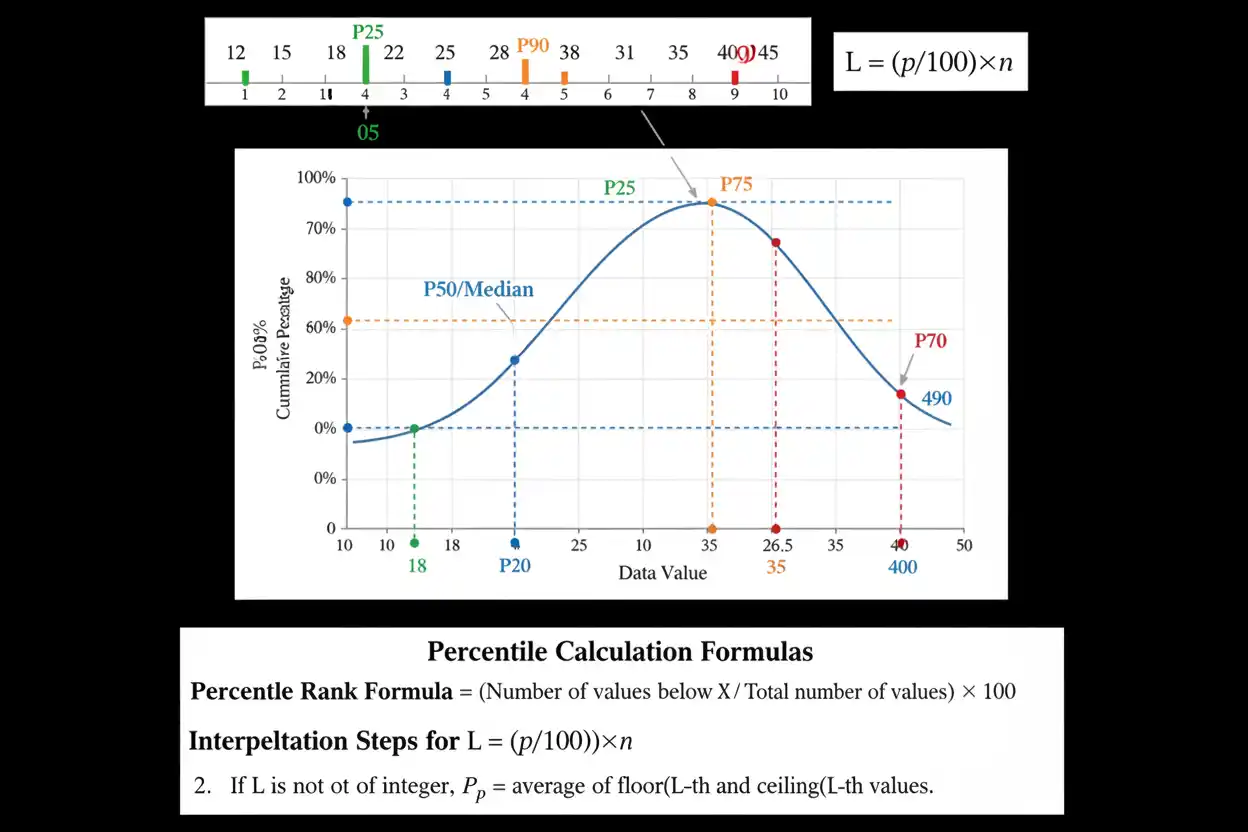
Percentiles describe the relative position of a value within an ordered data set or probability distribution by identifying the point at or below which a specified percentage of observations lies. The 25th percentile, for example, marks a value associated with approximately the lowest 25% of observations, while the 90th percentile identifies a point with approximately 90% of observations at or below it. Percentiles are therefore measures of position rather than measures of arithmetic average, and they remain useful even when a distribution is skewed or contains extreme observations. The 50th percentile corresponds to the median, while the 25th and 75th percentiles are commonly associated with the first and third quartiles. Calculating percentiles requires ordered data, but there is no single universally adopted finite-sample formula: nearest-rank methods, linear interpolation, and software-specific quantile conventions can produce slightly different results, especially in small samples. For continuous probability distributions, percentiles can instead be defined precisely through the cumulative distribution function. Understanding both the statistical meaning and the calculation convention is therefore essential whenever percentiles are compared, reported, or reproduced.
Percentiles are a core descriptive concept within core statistics and the wider Statistics & Probability framework. They connect ordered data with cumulative probability, while remaining distinct from inferential quantities such as p-values, which describe tail probabilities under a specified null model rather than positions within an observed distribution.
What Are Percentiles?
Percentiles divide an ordered distribution into one hundred relative positions.
The pth percentile is generally interpreted as a value associated with cumulative proportion:
p/100
For example, the 80th percentile is associated with cumulative proportion:
80/100 = 0.80
A practical interpretation is that approximately 80% of the observations are at or below that percentile value, depending on the precise finite-sample convention being used.
Similarly:
10th percentile → approximately 10% at or below
25th percentile → approximately 25% at or below
50th percentile → approximately 50% at or below
75th percentile → approximately 75% at or below
90th percentile → approximately 90% at or below
The values themselves remain in the original measurement units.
If heights are measured in centimeters, a height percentile is also expressed in centimeters. If the data are measured in seconds, the percentile value is measured in seconds.
Percentile vs Percentage
A percentage describes a proportion out of 100.
A percentile describes a position within an ordered distribution.
Suppose a student answers:
90%
of questions correctly.
That is a percentage score.
If the student is at the:
90th percentile
that instead means the score occupies a position around which approximately 90% of the comparison distribution lies at or below it.
A score of:
90%
does not automatically mean:
90th percentile
because percentile position depends on how everyone else performed.
If an examination is unusually difficult, a score of 70% could potentially correspond to a very high percentile. If nearly everyone scores above 90%, a 90% score could correspond to a much lower percentile.
Percentiles Require Ordered Data
To calculate sample percentiles, observations must first be arranged from smallest to largest.
Consider:
12, 4, 18, 7, 9
The ordered data are:
4, 7, 9, 12, 18
Percentile calculations use the ordered positions rather than the original recording sequence.
Failure to sort the observations before applying a rank formula can produce an entirely incorrect result.
The ordering requirement is one reason percentiles belong to the family of rank-based or quantile-based summaries.
Percentile Formula
There is no single universal percentile formula for every finite sample.
One common method is the nearest-rank method.
For percentile p in a sample of N ordered observations, calculate:
r = ⌈(p/100)N⌉
where:
⌈x⌉
means round x upward to the next integer.
The percentile is then the observation at rank:
r
with ranks beginning at 1.
Under this convention:
Pp = x₍ᵣ₎
where x₍ᵣ₎ is the rth ordered observation.
This method is easy to calculate but does not interpolate between observations.
Nearest-Rank Percentile Example
Consider the ordered data:
2, 4, 5, 7, 8, 10, 12, 15, 18, 21
There are:
N = 10
observations.
Find the 75th percentile.
Using the nearest-rank rule:
r = ⌈(75/100)(10)⌉
r = ⌈7.5⌉
r = 8
The eighth ordered observation is:
15
Therefore, under the nearest-rank convention:
75th percentile = 15
This answer is correct for that calculation convention.
Another legitimate percentile convention can produce a slightly different value.
Percentiles With Linear Interpolation
Many statistical systems use interpolation when the desired cumulative position lies between two observations.
A widely used interpolation convention calculates:
h = 1 + (n − 1)q
where:
q = p/100
and:
n = sample size.
If h is not an integer, write:
h = j + g
where j is the integer part and:
0 < g < 1
Then interpolate between ordered observations x₍ⱼ₎ and x₍ⱼ₊₁₎:
Pp = x₍ⱼ₎ + g[x₍ⱼ₊₁₎ − x₍ⱼ₎]
This approach produces a value between neighboring observations rather than always selecting one observed value.
Interpolated 75th Percentile Example
Use the same data:
2, 4, 5, 7, 8, 10, 12, 15, 18, 21
For the 75th percentile:
q = 0.75
There are:
n = 10
observations.
Calculate:
h = 1 + (10 − 1)(0.75)
h = 1 + 6.75
h = 7.75
Therefore:
j = 7
and:
g = 0.75
The seventh observation is:
x₍₇₎ = 12
The eighth is:
x₍₈₎ = 15
Interpolate:
P75 = 12 + 0.75(15 − 12)
P75 = 12 + 2.25
P75 = 14.25
Therefore, this interpolation convention gives:
75th percentile = 14.25
while the nearest-rank method gave:
15
Neither result is necessarily an error. They come from different percentile definitions.
Why Percentile Methods Differ
A finite sample contains only a limited number of observed positions.
Suppose:
n = 10
There is no actual observation occupying every one of the one hundred conceptual percentile positions.
Statistical conventions must therefore decide how percentile locations between observations should be represented.
One method chooses an actual observation.
Another interpolates between two observations.
Other methods place the sample observations at slightly different cumulative probabilities before interpolating.
Consequently, different software or textbooks may return different values for the same percentile in a small data set.
As samples become larger and distributions smoother, these differences often become relatively small.
Always State the Percentile Convention When Precision Matters
Suppose one calculation gives:
P75 = 14.25
while another gives:
P75 = 15
Without knowing the method, it is impossible to decide whether either result was calculated incorrectly.
For reproducible work, identify the method used by the software, calculator, statistical package, or analytical specification.
This is particularly important when percentile values define operational thresholds, clinical reference limits, service-level targets, admissions cutoffs, or other consequential boundaries.
A percentile should not be treated as method-independent when the sample is finite.
The 50th Percentile
The 50th percentile corresponds to the median.
For ordered data with an odd number of observations:
3, 6, 8, 10, 15
the middle value is:
8
Therefore:
P50 = 8
under standard median conventions.
For an even sample:
3, 6, 8, 10, 15, 20
the conventional median is:
(8 + 10)/2
= 9
Thus:
P50 = 9
under the ordinary interpolated median definition.
25th and 75th Percentiles
The 25th percentile is commonly associated with:
Q₁
the first quartile.
The 75th percentile is commonly associated with:
Q₃
the third quartile.
Thus:
Q₁ ≈ P25
Median = P50
Q₃ ≈ P75
The exact finite-sample values can depend on the quartile and percentile convention, but the conceptual relationship is stable.
These positions divide an ordered distribution into four broad portions.
Percentiles and Quartiles
Quartiles divide an ordered distribution into approximately four equal-probability sections.
Percentiles divide it conceptually into one hundred.
The relationship is:
Q₁ ↔ 25th percentile
Q₂ ↔ 50th percentile
Q₃ ↔ 75th percentile
Deciles similarly divide an ordered distribution into ten sections.
Therefore:
1st decile ↔ 10th percentile
5th decile ↔ 50th percentile
9th decile ↔ 90th percentile
These systems are different granularities of the broader quantile idea.
Percentiles and Quantiles
A quantile identifies the value corresponding to a cumulative probability q between:
0 and 1
A percentile expresses essentially the same cumulative position on a:
0 to 100
scale.
If:
q = 0.90
then the corresponding percentile is:
90th percentile
because:
p = 100q
Similarly:
25th percentile ↔ q = 0.25
50th percentile ↔ q = 0.50
95th percentile ↔ q = 0.95
The word quantile is therefore the more general probability-scale term.
Percentile Rank
A percentile value and a percentile rank are related but different.
A percentile asks:
What value corresponds to a specified cumulative position?
A percentile rank asks:
What cumulative position corresponds to a specified observed value?
For example:
“What is the 90th percentile?”
asks for a measurement value.
By contrast:
“What percentile is a score of 82?”
asks for a percentile rank.
These reverse the direction of the problem.
Simple Percentile Rank Formula
A simple empirical percentile-rank convention is:
Percentile rank = 100(B/N)
where:
- B = number of observations below the value
- N = total observations
Other conventions include observations equal to the score differently.
For data containing ties, a midpoint-rank convention is sometimes written:
Percentile rank = 100(B + 0.5E)/N
where:
- B = number below the score
- E = number equal to the score
- N = total observations
Again, percentile-rank definitions vary, so the convention should be stated when exact replication matters.
Percentile Rank Example
Suppose the ordered observations are:
40, 50, 60, 60, 60, 70, 80, 90
Find a midpoint-style percentile rank for:
x = 60
There are:
B = 2
observations below 60.
There are:
E = 3
observations equal to 60.
The total is:
N = 8
Therefore:
PR = 100(2 + 0.5×3)/8
PR = 100(3.5/8)
PR = 43.75
Under this convention, a score of 60 has percentile rank:
43.75
Another ranking convention could assign a different value because of how ties are handled.
Ties Matter in Percentile Ranks
Suppose many observations have exactly the same value.
There is no unique intuitive answer to:
“What percentage lies below this observation?”
versus:
“What percentage lies at or below it?”
For a repeated value, these quantities differ.
That is why percentile-rank conventions may use:
- strictly below,
- at or below,
- midpoint treatment of ties,
- averaged ranks.
The method should correspond to the intended interpretation.
Percentiles Do Not Mean Equal Numerical Spacing
The difference between the 10th and 20th percentiles need not equal the difference between the 70th and 80th percentiles.
Percentiles divide cumulative probability, not measurement distance.
Suppose a strongly right-skewed distribution has:
P10 = 2
P20 = 3
but:
P90 = 30
P100 near much larger values.
Equal ten-percent increments in cumulative position can correspond to dramatically different numerical distances.
Percentiles therefore describe relative rank, not equal intervals on the original scale.
Percentiles in Symmetric Distributions
For a distribution symmetric around μ, percentiles occur symmetrically around the center.
If:
P25 = μ − d
then:
P75 = μ + d
for an exactly symmetric distribution under the population quantile definition.
Likewise, the 10th and 90th percentiles are equally distant from the center.
This symmetry is particularly convenient for the normal distribution.
Skewed distributions do not generally have this property.
Percentiles in a Normal Distribution
Suppose:
X ~ N(μ, σ²)
To find the pth percentile, first obtain the standard normal quantile:
zₚ
satisfying:
P(Z ≤ zₚ) = p/100
Then transform it back to the original scale:
xₚ = μ + zₚσ
This gives an exact population percentile for the normal model, apart from numerical approximation used to evaluate zₚ.
For example, the 95th standard-normal percentile is approximately:
z₀.₉₅ ≈ 1.645
Therefore:
P95 ≈ μ + 1.645σ
for a normal distribution.
Normal Percentile Example
Suppose:
X ~ N(100, 15²)
Find the 90th percentile.
The standard normal 90th percentile is approximately:
z₀.₉₀ ≈ 1.282
Use:
x₉₀ = μ + z₀.₉₀σ
Therefore:
x₉₀ = 100 + 1.282(15)
x₉₀ = 100 + 19.23
x₉₀ ≈ 119.23
Thus, approximately 90% of this modeled population lies at or below:
119.23
and approximately 10% lies above it.
Finding a Percentile From a z-Score
Suppose a normal observation has:
z = 1.50
Its percentile rank is determined from the standard normal cumulative distribution:
Φ(1.50) ≈ 0.9332
Therefore, the observation is approximately at the:
93.32nd percentile
under the normal model.
In practical language, about:
93.32%
of the modeled distribution lies below or at that standardized location.
This illustrates the direct connection between cumulative probability and percentile position.
Percentiles and the Cumulative Distribution Function
For a continuous random variable X with cumulative distribution function:
F(x) = P(X ≤ x)
the q-quantile can be defined through the inverse CDF:
xq = F⁻¹(q)
where:
0 < q < 1
For percentile p:
q = p/100
so:
Pp = F⁻¹(p/100)
This is the cleanest population-level definition when F is continuous and strictly increasing.
In more general distributions, quantile definitions can require an infimum-based formulation because the CDF may have jumps or flat sections.
Percentiles in Discrete Distributions
Discrete distributions require special care because the CDF changes in jumps.
Suppose X takes only integer values.
There may be no x satisfying:
P(X ≤ x) = 0.90
exactly.
A common quantile definition chooses the smallest x such that:
F(x) ≥ 0.90
Thus, the 90th percentile can correspond to a cumulative probability larger than 90%.
This is a natural consequence of discrete probability mass rather than an error.
Percentiles of a Poisson Distribution
Suppose:
X ~ Poisson(λ)
The Poisson distribution is discrete, so its percentiles are integer count thresholds under common definitions.
For a desired cumulative probability q, a typical quantile definition finds the smallest integer k satisfying:
P(X ≤ k) ≥ q
Because the cumulative probability jumps from one integer count to the next, it generally cannot be forced to equal q exactly.
This differs from a continuous distribution, where many quantiles can be located more smoothly.
Percentiles and Outliers
Percentiles provide a natural way to describe extreme relative positions.
An observation above the:
99th percentile
lies above almost all of the reference distribution.
However, being extreme by percentile does not automatically make an observation invalid.
The detailed treatment of outliers distinguishes unusual values from confirmed errors and explains why context, data quality, and the assumed distribution matter.
A legitimate observation can occupy an extreme percentile simply because tail events genuinely occur.
Percentiles and the 1.5×IQR Rule
Because:
Q₁ ≈ P25
and:
Q₃ ≈ P75
the interquartile range is closely connected to percentiles:
IQR = P75 − P25
under a consistent quartile convention.
Outlier fences then extend beyond those percentile-based quartiles:
Lower fence = Q₁ − 1.5(IQR)
Upper fence = Q₃ + 1.5(IQR)
These fences are not themselves fixed percentile levels across all distributions.
Their corresponding cumulative probabilities depend on distribution shape.
Percentiles and P-Values
Percentiles and p-values both involve cumulative probability, but they answer different questions.
A percentile locates a value within a distribution.
A p-value measures the probability, under a null model, of obtaining a test statistic at least as extreme as the observed one.
Suppose an upper-tailed test statistic lies at the:
98th percentile
of its null reference distribution.
Then:
F(t_obs) = 0.98
and the upper-tail p-value is:
p = 1 − 0.98
p = 0.02
Thus, the percentile gives cumulative position, while the p-value gives the relevant tail area.
Two-Sided Tests and Percentiles
Suppose a symmetric null distribution produces:
z = 1.96
The standard normal cumulative probability is approximately:
Φ(1.96) ≈ 0.975
Therefore, +1.96 lies at approximately the:
97.5th percentile
and:
−1.96
lies near the:
2.5th percentile.
The probability in the two tails combined is:
2.5% + 2.5% = 5%
which corresponds to a two-sided:
p ≈ 0.05
This is why the 2.5th and 97.5th percentiles appear in standard two-sided 95% normal procedures.
Percentiles and Odds Formats
A cumulative probability can be converted to odds formats when an odds representation is genuinely useful.
Suppose an observation lies at the:
90th percentile
of a continuous reference distribution.
Its lower cumulative probability is:
0.90
while the upper-tail probability is:
0.10
If the event of interest is:
“exceed this threshold”
then the relevant probability is:
10%
not 90%.
Fair decimal odds corresponding to a 10% upper-tail probability would be:
1/0.10 = 10.00
The direction of the event must therefore be identified before translating a percentile into another probability representation.
Percentiles in Skewed Distributions
Percentiles are especially useful for skewed data because they depend on ordered position rather than arithmetic distance from the mean.
Suppose a distribution has:
P50 = 20
P75 = 30
P90 = 70
P99 = 500
The rapidly increasing gaps indicate a long upper tail.
A mean and standard deviation alone may not communicate this structure clearly.
Reporting multiple percentiles can reveal how the distribution changes from its center into its tails.
Percentiles Are Resistant to Extreme Magnitudes
Suppose the largest observation changes from:
100
to:
1,000,000
Many lower percentiles may remain unchanged if the rank ordering of the remaining data does not change.
The arithmetic mean, by contrast, could shift dramatically.
This rank-based resistance makes percentiles useful in distributions containing large legitimate extremes.
However, very high percentiles such as P99 can themselves be sensitive to tail observations and sample size.
Extreme Percentiles Need More Data
Estimating:
P50
requires information near the center of the distribution.
Estimating:
P99.9
requires accurate information about an extremely small upper-tail region.
In a sample of:
n = 100
there is very little direct information about the 99.9th percentile.
Even:
P99
can be unstable in small samples.
Reliable estimation of extreme percentiles often requires much larger data sets, tail modeling, or additional assumptions.
A reported percentile can therefore have substantial sampling uncertainty even when the arithmetic calculation appears simple.
Percentiles and Sample Size
Suppose:
n = 20
Then each ordered observation represents a relatively large portion of the empirical distribution.
Small changes in one observation can move estimated percentiles noticeably.
With:
n = 100,000
central percentile estimates can usually be much more stable, assuming the observations adequately represent the target population.
Large sample size does not eliminate sampling bias, dependence, or nonrepresentative data, but it can reduce random uncertainty in percentile estimates.
Sample Percentiles Are Statistics
A percentile calculated from sample data is a sample statistic.
It estimates a corresponding population quantile or percentile.
Different random samples from the same population generally produce different sample percentiles.
For example, one random sample might give:
sample P90 = 72
while another gives:
sample P90 = 75
Neither must equal the true population 90th percentile exactly.
This sampling variability is distinct from differences caused by competing percentile-calculation conventions.
Population Percentiles
For a fully specified population distribution, a percentile is a population characteristic.
For a continuous CDF F:
Pp = F⁻¹(p/100)
For example, if a theoretical distribution has known parameters, the 95th percentile can be calculated directly from the model.
A population percentile is conceptually fixed.
A sample percentile is an estimate that varies from sample to sample.
Percentiles in Performance Data
Suppose a response time has:
P50 = 100 ms
P90 = 180 ms
P99 = 500 ms
This tells us much more about the upper tail than the median alone.
The interpretation is approximately:
50% at or below 100 ms
90% at or below 180 ms
99% at or below 500 ms
under the relevant empirical or modeled percentile convention.
The large gap from P90 to P99 indicates that the slowest portion of the distribution extends substantially farther than the central observations.
Percentiles in Growth and Reference Data
Percentiles are frequently used to compare an individual’s measurement with a reference population.
Suppose a value lies at the:
70th percentile.
This means its position is higher than roughly 70% of the reference distribution under the specified percentile convention.
It does not mean:
70% better
or:
70% larger
than the average.
Percentiles measure rank position, not proportional difference.
The identity and representativeness of the reference population are therefore essential to interpretation.
Percentile Changes Do Not Equal Percentage Changes
Suppose a measurement moves from the:
40th percentile
to the:
60th percentile.
That is a change of:
20 percentile points.
It is not automatically a:
50% increase
in the underlying measurement.
The numerical change in the original variable depends on the distribution.
If the distribution is dense near the center, a small raw-value change could move many percentile points. In a sparse tail, a large raw-value change might move only a few.
Percentile Points vs Percent Change
The difference between:
30th percentile
and:
50th percentile
is:
20 percentile points.
The relative increase in the percentile number would mathematically be:
(50 − 30)/30
≈ 66.7%
but this percentage usually has little meaningful statistical interpretation.
Percentile positions are ranks on a cumulative scale.
Reporting the difference in percentile points is generally clearer.
Percentiles and Nonlinear Relationships
Percentile transformations are nonlinear.
The difference in raw values between adjacent percentile positions depends on the local density of the distribution.
This is important when interpreting models such as polynomial regression.
A regression may model a conditional mean relationship, while percentile or quantile methods describe different parts of the conditional distribution.
A curved mean relationship should not be interpreted as automatically describing how every percentile of the response changes.
Mean Regression vs Percentile-Based Questions
Ordinary least-squares regression typically models:
E(Y|X)
the conditional mean response.
A percentile-based question might instead ask:
What is the 90th percentile of Y conditional on X?
These are different targets.
The conditional mean can rise while upper and lower percentiles change at different rates.
Specialized quantile-regression methods can model conditional quantiles directly, but the core percentile concept remains the ordered probability position described here.
Percentiles Can Be Equal
In discrete data or data with many ties, several percentiles can have the same numerical value.
Suppose:
0, 0, 0, 0, 1, 1, 1, 1, 1, 1
Many lower percentile positions can map to:
0
while many upper positions map to:
1
That is perfectly valid.
Percentiles divide cumulative probability or rank position, not necessarily the numerical measurement scale into distinct values.
Percentiles Need Not Be Observed Values
Under interpolation methods, a sample percentile can lie between two observed values.
Suppose neighboring observations are:
12
and:
15
An interpolated percentile could be:
14.25
even though:
14.25
does not appear anywhere in the sample.
This is analogous to the median of an even-sized sample, which can also lie between observed values.
Under nearest-rank methods, by contrast, percentiles are always selected from actual observations.
Minimum and Maximum Percentiles
Definitions at the exact endpoints:
0th percentile
and:
100th percentile
vary by mathematical and software convention.
In many descriptive systems:
P0 = minimum
P100 = maximum
Other formal quantile definitions require careful endpoint treatment.
For practical sample reporting, the minimum and maximum are often treated as the 0th and 100th percentile endpoints, but it is useful to recognize that quantile definitions can differ at boundaries.
Common Percentiles
Certain percentiles appear frequently because they summarize important regions of a distribution.
The 25th, 50th, and 75th percentiles describe quartile structure. The 5th and 95th percentiles describe broad lower and upper reference regions. The 90th, 95th, 99th, and 99.9th percentiles are often used when upper-tail behavior matters.
The correct percentile depends on the question.
There is nothing inherently universal about using P95 instead of P90 or P99.
The chosen level should reflect the decision or descriptive objective.
Percentiles and Missing Data
Missing values should not automatically be assigned:
0
before calculating percentiles.
Doing so inserts artificial observations into the ordered distribution and can alter many percentile positions.
If incomplete observations are excluded, the percentile calculation applies to the remaining data.
However, if missingness is systematic, the observed distribution itself may no longer represent the target population.
Percentiles are only as representative as the data used to estimate them.
Percentiles and Weighted Data
Some analyses assign different weights to observations.
A weighted percentile uses cumulative weight rather than simple observation count.
Suppose one observation represents:
1 person
while another survey record represents:
1,000 people
Treating both as equally weighted can give the wrong population percentile.
Weighted percentile methods accumulate the statistical weights and identify the value corresponding to the desired proportion of total weight.
As with unweighted percentiles, exact interpolation conventions can differ.
Percentiles and Grouped Data
When only grouped frequency intervals are available, exact raw-data percentiles may be impossible to recover.
Suppose data are reported only as:
0–10: 20 observations
10–20: 50 observations
20–30: 30 observations
The 50th percentile lies somewhere within the:
10–20
class because cumulative frequency passes 50% there.
An interpolated grouped-data estimate can be calculated by assuming a distribution within the class.
Because the original individual values are unavailable, the result is approximate.
Percentile From Grouped Data
A common grouped-data interpolation formula is:
Pp = L + [(pN/100 − CF)/f]w
where:
- L = lower boundary of the percentile class
- N = total frequency
- CF = cumulative frequency before that class
- f = frequency within the percentile class
- w = class width
This method assumes observations are distributed sufficiently evenly within the relevant interval for linear interpolation to be useful.
It should therefore be described as an estimate rather than an exact raw-data percentile.
Grouped Percentile Example
Suppose:
| Interval | Frequency |
|---|---|
| 0–10 | 20 |
| 10–20 | 50 |
| 20–30 | 30 |
Then:
N = 100
Find:
P50
The target cumulative position is:
50
The first class contains positions through:
20
The second class contains positions:
21 through 70
so the percentile class is:
10–20
Using:
L = 10
CF = 20
f = 50
w = 10
we obtain:
P50 ≈ 10 + (50 − 20)/50
P50 ≈ 10 + 6
P50 ≈ 16
This is an interpolated estimate based on grouped information.
Percentiles and Data Transformations
If a transformation is strictly increasing, percentile ranks are preserved.
Suppose:
Y = aX + b
with:
a > 0
Then the pth percentile transforms as:
Pp(Y) = aPp(X) + b
For example, converting temperatures or lengths through a positive linear transformation preserves ordering.
A value at the:
90th percentile
before the transformation remains at the:
90th percentile
afterward.
The numerical percentile value changes, but its rank does not.
Decreasing Transformations Reverse Percentile Positions
If a transformation is strictly decreasing, the ordering reverses.
For example:
Y = −X
turns large X values into small Y values.
An observation at a high percentile of X therefore becomes associated with a low percentile of Y.
This is an important reminder that percentile rank is fundamentally based on ordering.
Positive monotonic transformations preserve that ordering; decreasing transformations reverse it.
Percentiles and Standardization
Suppose:
z = (x − μ)/σ
with:
σ > 0
This is a strictly increasing linear transformation.
Therefore, percentile ranks are preserved.
If x is at the:
95th percentile
of X, its z-score is at the:
95th percentile
of the standardized distribution.
For normally distributed data:
95th percentile ↔ z ≈ 1.645
This allows direct movement between original measurement units and standardized percentile positions.
Percentiles Are Not Probabilities of Individual Values
Suppose:
P90 = 120
This does not mean:
P(X = 120) = 0.90
Instead, it refers to cumulative probability:
P(X ≤ 120) ≈ 0.90
under the relevant population or empirical convention.
For a continuous distribution:
P(X = 120) = 0
even though 120 can be the 90th percentile.
Confusing point probability with cumulative probability is a common error.
Percentiles Are Not Measures of Causation
Suppose one group has a higher 90th percentile than another.
This shows a difference in distributional position.
It does not establish why the difference exists.
Possible explanations include:
- causal effects,
- population composition,
- sampling variation,
- measurement differences,
- confounding.
Percentiles are descriptive statistics unless embedded in a design that supports stronger causal conclusions.
Comparing Percentiles Across Groups
Suppose:
Group A P90 = 80
Group B P90 = 100
The correct descriptive conclusion is that the 90th-percentile value is 20 units higher in Group B.
That does not mean every observation in Group B is 20 units higher.
Nor does it mean Group B is universally better or worse.
Percentile comparisons summarize specific regions of each distribution.
Comparing P50, P75, P90, and P99 together can reveal whether group differences occur throughout the distribution or primarily in one tail.
Percentiles Can Reveal Distribution Shape
Consider:
P10 = 10
P25 = 20
P50 = 30
P75 = 40
P90 = 50
The approximately regular spacing suggests a relatively balanced central distribution.
Now consider:
P10 = 10
P25 = 20
P50 = 30
P75 = 50
P90 = 120
The rapidly expanding upper gaps suggest substantial right-tail extension.
Percentile spacing provides useful shape information without requiring a particular probability model.
Percentiles Do Not Fully Describe a Distribution
Two distributions can share:
P25
P50
P75
while differing substantially in:
- tails,
- local clusters,
- gaps,
- extreme values.
Likewise, reporting P95 alone does not reveal what happens below that threshold.
Percentiles are powerful summaries, but a complete analysis may require:
- several percentile levels,
- graphical displays,
- measures of center,
- measures of spread,
- an appropriate statistical model.
Common Percentile Mistakes
A frequent mistake is failing to sort the data before calculating percentiles.
Another is assuming there is only one universally correct finite-sample percentile formula.
A third is confusing a percentile with a percentage score.
Another common error is interpreting the 90th percentile as meaning an observation is “90% greater” than average.
Analysts may also confuse a percentile value with percentile rank, even though one maps cumulative position to a value and the other maps a value to cumulative position.
Another error is assuming that equal percentile-point differences correspond to equal numerical distances.
It is also incorrect to assume that a percentile must always equal an observed sample value because interpolation methods can produce intermediate values.
Finally, extreme sample percentiles should not be interpreted as highly precise when the available sample contains little information about the tail.
How to Calculate Percentiles Step by Step
First, arrange all observations from smallest to largest.
Second, choose the percentile level p between 0 and 100.
Third, identify the calculation convention being used. For nearest-rank percentiles:
r = ⌈(p/100)N⌉
and select the rth observation.
For a common linear interpolation method:
h = 1 + (n − 1)(p/100)
and interpolate between the neighboring ordered observations when h is not an integer.
Finally, report both the percentile value and, when reproducibility matters, the method used.
The calculation should never mix ranking conventions midway through the same analysis.
Full Worked Example
Consider the ordered sample:
3, 5, 7, 9, 12, 15, 18, 22, 27, 35, 44
There are:
n = 11
observations.
Find the 80th percentile using:
h = 1 + (n − 1)q
where:
q = 0.80
Calculate:
h = 1 + 10(0.80)
h = 9
Because h is exactly an integer, no interpolation is required.
The ninth ordered observation is:
27
Therefore:
P80 = 27
under this interpolation convention.
Approximately 80% of the distribution is associated with values at or below this position according to the selected sample-quantile definition.
Worked Example Requiring Interpolation
Using the same data, find:
P85
Now:
q = 0.85
Calculate:
h = 1 + 10(0.85)
h = 9.5
Therefore, the desired position lies halfway between the ninth and tenth observations.
Those observations are:
x₍₉₎ = 27
x₍₁₀₎ = 35
Interpolate:
P85 = 27 + 0.5(35 − 27)
P85 = 27 + 4
P85 = 31
Therefore:
85th percentile = 31
under this method.
How to Report Percentiles
A clear report identifies the measurement and percentile.
For example:
Median response time (P50) = 120 ms; P90 = 210 ms; P99 = 640 ms.
When the calculation convention materially affects the values, add the method.
For example:
P90 was calculated using linear interpolation with h = 1 + (n − 1)q.
If percentiles come from a theoretical model rather than raw empirical observations, state that distinction as well.
A modeled percentile and an empirical sample percentile need not be identical.
Frequently Asked Questions About Percentiles
What are percentiles?
Percentiles identify positions within an ordered distribution. The pth percentile corresponds to a value associated with cumulative proportion p/100.
What does the 90th percentile mean?
It means the percentile value is located so that approximately 90% of the reference distribution lies at or below it under the specified convention.
Is the 50th percentile the median?
Yes. The 50th percentile corresponds to the median under standard definitions.
What is the 25th percentile?
The 25th percentile corresponds conceptually to the first quartile.
What is the 75th percentile?
The 75th percentile corresponds conceptually to the third quartile.
What is the nearest-rank percentile formula?
A common formula is:
r = ⌈(p/100)N⌉
The percentile is the rth ordered observation.
Why do calculators sometimes give different percentiles?
Different systems can use different ranking and interpolation conventions for finite samples.
Is one percentile formula universally correct?
No. Several established finite-sample quantile conventions exist. The chosen method should be stated when exact reproducibility matters.
What is interpolation in percentile calculations?
Interpolation estimates a percentile value between neighboring ordered observations when the required rank is fractional.
Can a percentile be a value not present in the sample?
Yes. Interpolated percentiles can lie between observed values.
Are percentiles the same as percentages?
No. A percentage measures a proportion, while a percentile measures relative position within an ordered distribution.
Does scoring 90% mean being at the 90th percentile?
No. Percentile rank depends on the score distribution of the comparison population.
What is percentile rank?
Percentile rank describes the cumulative position of a specified observed value rather than finding the value associated with a specified percentile.
How are ties handled in percentile ranks?
Different conventions exist. Some use the number below the score, some include equal scores, and some assign tied observations a midpoint rank.
Are quartiles percentiles?
Yes conceptually: Q₁ corresponds to P25, Q₂ to P50, and Q₃ to P75.
Are deciles percentiles?
Yes. Each decile corresponds to a multiple of ten percentile points.
What is the relationship between quantiles and percentiles?
A quantile uses a probability scale from 0 to 1. A percentile uses a scale from 0 to 100:
percentile = 100 × quantile probability.
How do you find a normal-distribution percentile?
Use:
xₚ = μ + zₚσ
where zₚ is the standard-normal quantile associated with cumulative probability p/100.
What z-score is the 95th percentile?
Approximately:
z = 1.645
for the 95th percentile of a standard normal distribution.
What percentile is z = 1.96?
Approximately:
97.5th percentile
of the standard normal distribution.
Can a discrete distribution have an exact 90th-percentile cumulative probability?
Not necessarily. Because discrete CDFs jump, the usual quantile may be the smallest value whose cumulative probability is at least 90%.
How are percentiles related to p-values?
A percentile gives cumulative position within a reference distribution. A p-value uses the appropriate tail probability beyond an observed test statistic under a null model.
Can percentiles identify outliers?
Extreme percentile positions can indicate unusual observations, but they do not automatically establish that a value is erroneous.
Are percentiles affected by extreme values?
Central percentiles are generally resistant to the precise magnitudes of isolated extreme observations, although very high or low percentiles naturally depend on tail data.
Why are P99 and P99.9 difficult to estimate?
They depend on very small tail fractions, so large samples or additional modeling may be required for stable estimates.
Can several percentiles have the same value?
Yes, especially in discrete data or samples with many repeated observations.
Do equal percentile differences mean equal measurement differences?
No. Percentiles divide cumulative probability, not numerical distance on the original scale.
Do percentiles change under unit conversions?
A strictly increasing linear conversion changes the numerical percentile values but preserves percentile ranks.
What is the main rule when comparing percentiles?
Use the same reference population, data definition, and percentile-calculation convention before interpreting numerical differences.




