


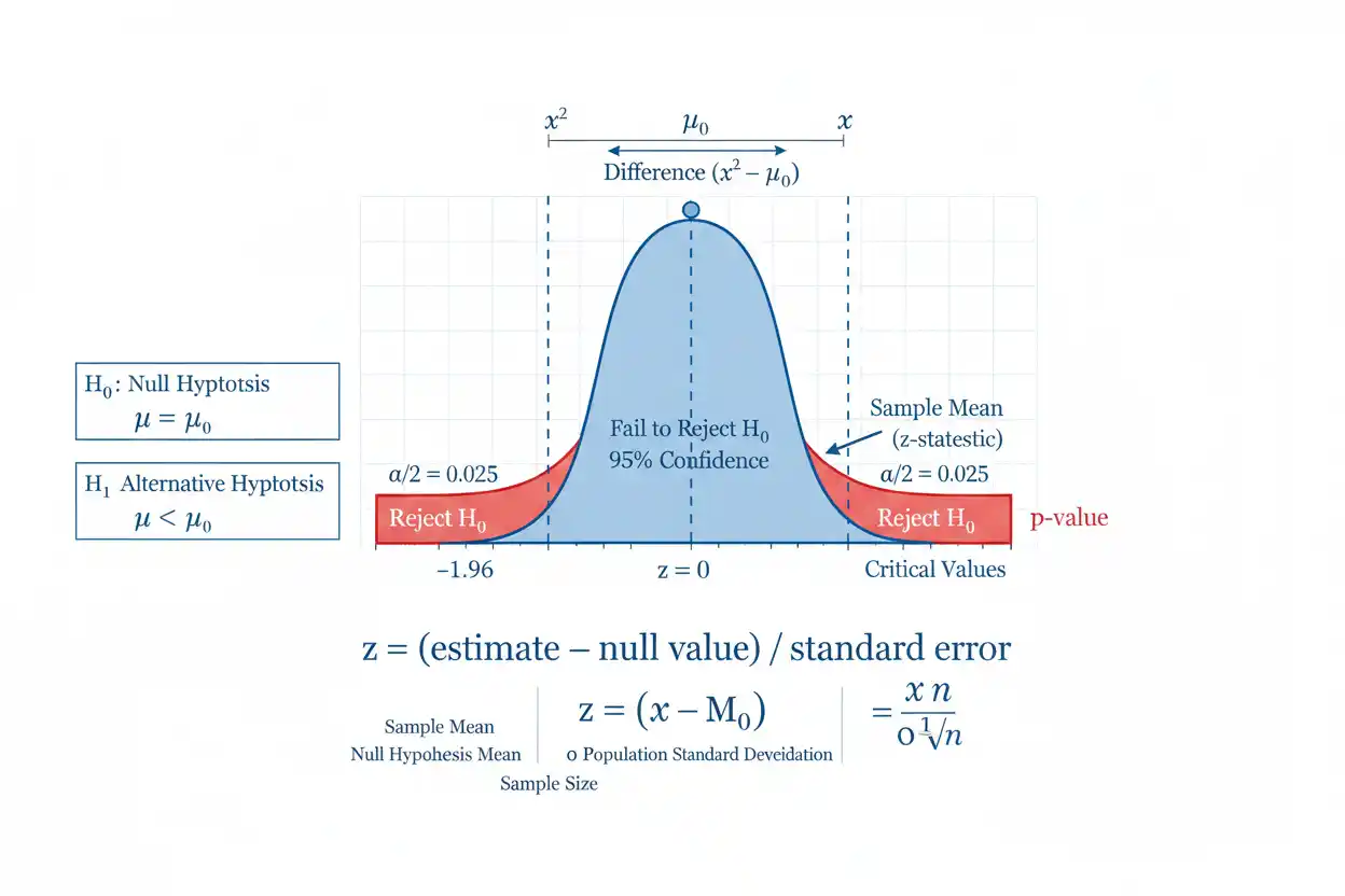
A z-test is a statistical hypothesis test that measures how far an observed sample estimate lies from a value specified by the null hypothesis after the difference has been divided by an appropriate standard error. The resulting z statistic is evaluated against the standard normal distribution, allowing the analyst to calculate a p-value or compare the result with critical values such as ±1.96 for a two-sided 5% significance test. For a population mean, the classical one-sample z-test is most directly applicable when the population standard deviation is genuinely known and the sampling distribution of the mean is normal or adequately approximated by a normal distribution. Related z procedures are also widely used for proportions because their large-sample sampling distributions can often be approximated by normal distributions even though the underlying individual observations are binary. The basic logic remains the same across these applications: define a null hypothesis, calculate the difference between the observed estimate and the null value, express that difference in standard-error units, and determine whether such a standardized result would be unusually extreme if the null model were correct.
The z-test belongs to the inferential methods within core statistics and the broader Statistics & Probability framework. Its standardized test statistic is closely related to the z-score, but the denominator in a hypothesis test is typically the standard error of an estimator rather than the standard deviation of individual observations, making this distinction essential for correct calculation and interpretation.
What Is a z-Test?
A z-test compares an observed statistic with a hypothesized population value using a standard normal reference distribution.
Its general structure is:
z = (Observed estimate − Null value) / Standard error
The numerator measures the raw discrepancy from the null hypothesis, while the denominator measures how much the estimate would ordinarily fluctuate across repeated samples under the statistical model.
A result such as:
z = 0.4
means the estimate is only 0.4 standard errors from the null value.
A result such as:
z = 3
means the estimate is three standard errors from the null value, which is considerably more unusual under a standard normal null model.
The z-test therefore evaluates a discrepancy relative to statistical precision rather than considering the raw difference alone.
z-Test Formula for a Population Mean
For a one-sample mean when the population standard deviation σ is known, the z-test statistic is:
z = (x̄ − μ₀)/(σ/√n)
where:
- x̄ = sample mean
- μ₀ = population mean specified by H₀
- σ = known population standard deviation
- n = sample size
- σ/√n = standard error of the sample mean
A common two-sided hypothesis is:
H₀: μ = μ₀
H₁: μ ≠ μ₀
Under H₀ and the required assumptions, the z statistic follows:
Z ~ N(0,1)
either exactly or approximately depending on the sampling model.
Why the Denominator Is σ/√n
Individual observations may vary with population standard deviation:
σ
but a sample mean varies much less because it averages n observations.
For independent observations with population variance:
σ²
the variance of the sample mean is:
Var(X̄) = σ²/n
Therefore:
SD(X̄) = σ/√n
This quantity is the standard error of the sample mean.
The z-test compares:
x̄ − μ₀
with this sampling variability, not with the variation of one individual observation.
That distinction is why the denominator is:
σ/√n
rather than simply:
σ.
One-Sample z-Test Example
Suppose a process is believed to have population mean:
μ₀ = 50
and the population standard deviation is known to be:
σ = 8
A random sample of:
n = 64
independent observations has mean:
x̄ = 53
Test:
H₀: μ = 50
against:
H₁: μ ≠ 50
First calculate the standard error:
SE = σ/√n
SE = 8/√64
SE = 8/8
SE = 1
Now calculate the z statistic:
z = (53 − 50)/1
z = 3
The observed sample mean is therefore:
3 standard errors above the null mean.
Calculating the p-Value
For a two-sided z-test:
p = 2P(Z ≥ |zobs|)
With:
zobs = 3
the upper-tail standard-normal probability is approximately:
P(Z ≥ 3) ≈ 0.00135
Therefore:
p ≈ 2(0.00135)
p ≈ 0.00270
At:
α = 0.05
we have:
p < α
so the test rejects:
H₀: μ = 50.
The result provides strong statistical evidence that the population mean differs from 50 under the z-test model and assumptions.
It does not by itself explain why the mean differs or establish causal interpretation.
Interpreting the Worked Example
The sample mean exceeds the null value by:
53 − 50 = 3 units.
Because the standard error is only:
1 unit
that three-unit raw difference represents:
3 standard errors.
If the standard error had instead been:
10
the same three-unit difference would produce:
z = 0.3
and provide very little evidence against the null value.
Statistical evidence therefore depends on both:
effect magnitude
and:
uncertainty.
A raw difference cannot be interpreted properly without knowing its scale relative to sampling variability.
Two-Sided z-Test
A two-sided test considers departures from the null in either direction.
The hypotheses are:
H₀: μ = μ₀
H₁: μ ≠ μ₀
For a significance level:
α = 0.05
the standard-normal critical values are approximately:
−1.96 and +1.96
The rejection regions are:
z < −1.96
or:
z > 1.96
Equivalently:
|z| > 1.96
leads to rejection at the 5% two-sided level.
This rule works because approximately 95% of a standard normal distribution lies between −1.96 and +1.96, leaving approximately 2.5% in each tail.
Upper-Tailed z-Test
An upper-tailed test is appropriate when only values above the null threshold are relevant to the pre-specified alternative.
The hypotheses can be written:
H₀: μ = μ₀
H₁: μ > μ₀
For:
α = 0.05
the upper-tail critical value is approximately:
z = 1.645
Therefore:
z > 1.645
falls in the rejection region.
The p-value is:
p = P(Z ≥ zobs)
for a positive observed statistic.
A one-sided direction should be determined from the research question before observing the result rather than chosen afterward because the sample mean happens to fall on one side of μ₀.
Lower-Tailed z-Test
A lower-tailed test evaluates:
H₀: μ = μ₀
against:
H₁: μ < μ₀
At:
α = 0.05
the critical value is approximately:
z = −1.645
so:
z < −1.645
falls in the rejection region.
The corresponding p-value is:
p = P(Z ≤ zobs)
A strongly negative z statistic provides evidence in the lower-tail direction.
The sign therefore matters when the alternative is directional.
Common z Critical Values
Several critical values appear repeatedly in standard-normal inference:
| Test or central confidence level | Critical z |
|---|---|
| 90% two-sided | ±1.645 |
| 95% two-sided | ±1.960 |
| 98% two-sided | ±2.326 |
| 99% two-sided | ±2.576 |
| 5% one-sided | 1.645 |
| 2.5% one-sided | 1.960 |
| 1% one-sided | 2.326 |
These values come from quantiles of:
N(0,1)
rather than from arbitrary statistical conventions.
For example:
P(Z ≤ 1.96) ≈ 0.975
so approximately:
2.5%
lies above 1.96.
Critical-Value Method
The critical-value method compares the observed statistic with a pre-defined rejection boundary.
For a two-sided test with:
α = 0.05
reject H₀ if:
|zobs| > 1.96
In the worked example:
zobs = 3
and:
3 > 1.96
so H₀ is rejected.
This produces the same decision as comparing:
p ≈ 0.0027
with:
α = 0.05.
The p-value method communicates how extreme the result is continuously, whereas the critical-value method emphasizes whether the result enters a specified rejection region.
p-Value Method
The p-value is calculated from the null reference distribution.
For a two-sided z-test:
p = 2P(Z ≥ |zobs|)
For an upper-tailed test:
p = P(Z ≥ zobs)
For a lower-tailed test:
p = P(Z ≤ zobs)
The decision rule is usually:
If p ≤ α → reject H₀
If p > α → fail to reject H₀
The significance level α should ordinarily be chosen before the data are used for the final hypothesis decision.
What a p-Value Means
Suppose:
p = 0.0027.
This means that under H₀ and the statistical assumptions of the z-test, a test statistic at least as extreme as the observed result would occur with probability approximately:
0.27%
according to the relevant two-sided tail definition.
It does not mean:
“There is a 0.27% probability that H₀ is true.”
It also does not mean:
“There is a 99.73% probability that H₁ is true.”
The p-value is calculated conditional on the null model; it is not a posterior probability assigned to the hypotheses themselves.
Failing to Reject the Null Hypothesis
Suppose a test gives:
z = 0.8
and:
p ≈ 0.424
for a two-sided alternative.
At:
α = 0.05
we would:
fail to reject H₀.
This does not prove that the population parameter equals the null value.
The data may simply contain insufficient evidence to distinguish the observed difference from normal sampling variation.
A non-significant result can occur because the true effect is small, the sample is too small, population variation is large, or the estimate happens to fall near the null by chance.
Failure to reject and proof of equality are not the same conclusion.
z-Test Confidence Interval
The one-sample known-σ z-test is closely connected with the confidence interval:
x̄ ± z*σ/√n
For the earlier example:
x̄ = 53
σ = 8
n = 64
At 95% confidence:
z* = 1.96
and:
SE = 1
Therefore:
53 ± 1.96(1)
gives:
53 ± 1.96
or:
(51.04, 54.96)
The null value:
50
lies outside this interval.
That agrees with the two-sided z-test decision at:
α = 0.05.
Relationship Between the Confidence Interval and Test
For a standard two-sided procedure, a null value is rejected at significance level α when it lies outside the corresponding:
100(1 − α)%
confidence interval.
Thus, at:
α = 0.05
a null value outside the 95% interval corresponds to rejection.
The confidence interval often provides more useful information because it shows the range of population means reasonably compatible with the data under the procedure.
A p-value shows evidence against one null value.
The interval displays effect magnitude and uncertainty over a continuum of possible parameter values.
z-Test vs z-Score
A z-score for one observation is:
z = (x − μ)/σ
A z-test statistic for a sample mean is:
z = (x̄ − μ₀)/(σ/√n)
The first asks:
How unusual is one observation relative to individual population variability?
The second asks:
How unusual is a sample mean relative to the sampling variability of sample means?
These are different questions.
For large n, the denominator σ/√n can be much smaller than σ, so the same raw numerical difference can yield a much larger hypothesis-test z statistic.
z-Score vs z-Test Example
Suppose:
μ = 100
σ = 20.
An individual observation:
x = 104
has:
z = (104 − 100)/20
z = 0.2
Therefore, the observation is only 0.2 standard deviations above the mean.
Now suppose:
n = 100
and:
x̄ = 104.
The standard error of the mean is:
20/√100
= 2
so the z-test statistic is:
z = (104 − 100)/2
= 2
The sample mean is two standard errors above μ even though an individual score of 104 is only 0.2 standard deviations above μ.
z-Test vs t-Test
The classical distinction between a z-test and t-test for a population mean concerns whether the population standard deviation is known.
A mean z-test uses:
z = (x̄ − μ₀)/(σ/√n)
A one-sample t-test uses:
t = (x̄ − μ₀)/(s/√n)
where:
s
estimates the unknown population standard deviation.
Estimating σ introduces additional uncertainty, so the t statistic uses Student’s t distribution rather than an exact standard normal reference distribution under the classical normal model.
In practical work, population σ is often unknown, making the t-test more appropriate for ordinary mean inference.
Is a z-Test Automatically Correct for a Large Sample?
A common rule says:
“Use z when n ≥ 30.”
This is overly simplistic.
If population σ is unknown, replacing it with sample s changes the theoretical procedure. For large samples, t and z critical values become numerically very similar, so the practical difference can be tiny, but this does not make the classical distinction disappear.
Moreover, a large sample does not automatically validate:
- independence,
- representative sampling,
- correct standard errors,
- absence of influential dependence,
- an appropriate probability model.
Sample size can support normal approximations, but it cannot fix every statistical assumption.
When Is a One-Sample Mean z-Test Appropriate?
A classical one-sample mean z-test is most defensible when:
- the target parameter is a population mean,
- population σ is known from a credible source rather than estimated from the same sample,
- observations are independent or the standard-error model correctly accounts for dependence,
- the sampling distribution of x̄ is normal or adequately approximated by normality,
- the sampling mechanism supports the desired population inference.
If the population is itself normal and observations are independent:
X̄
is exactly normal for every sample size.
For non-normal populations, large-sample central-limit behavior can provide an approximation under suitable conditions.
Known Population Standard Deviation Is Uncommon
In many real data analyses, σ is not truly known.
A historical estimate of standard deviation is still an estimate unless the inferential model explicitly treats it as fixed and known.
Using a sample estimate s while calling the resulting procedure an exact known-σ z-test hides uncertainty.
For ordinary one-sample mean analysis with unknown σ, a t procedure generally represents that uncertainty more directly.
This distinction matters especially in small samples, where t critical values can be substantially larger than standard-normal critical values.
One-Sample Proportion z-Test
Z procedures are also frequently used to test population proportions.
Suppose:
p
is an unknown population proportion and:
p₀
is the null value.
The sample proportion is:
p̂ = x/n
where x is the number of successes.
Under H₀:
H₀: p = p₀
the null standard error is:
SE₀ = √[p₀(1 − p₀)/n]
and the z statistic is:
z = (p̂ − p₀)/SE₀
or:
z = (p̂ − p₀)/√[p₀(1−p₀)/n]
This is typically a large-sample normal approximation to the binomial sampling distribution.
One-Proportion z-Test Example
Suppose the null hypothesis is:
H₀: p = 0.40
A sample contains:
n = 200
observations and:
x = 96
successes.
The sample proportion is:
p̂ = 96/200
p̂ = 0.48
The null standard error is:
SE₀ = √[(0.40)(0.60)/200]
= √(0.24/200)
= √0.0012
≈ 0.03464
Therefore:
z = (0.48 − 0.40)/0.03464
z ≈ 2.31
The two-sided p-value is approximately:
p ≈ 0.021
At α = 0.05, this provides evidence against:
p = 0.40
under the large-sample proportion z-test model.
Why the Null Proportion Appears in the Standard Error
For hypothesis testing:
H₀: p = p₀
the null hypothesis specifies the probability model that determines the sampling variability of p̂.
Therefore:
Var₀(p̂) = p₀(1 − p₀)/n
and:
SE₀ = √[p₀(1−p₀)/n]
This differs from a common confidence-interval standard error, which may use:
p̂
rather than:
p₀.
The hypothesis test and confidence interval must therefore be paired carefully when using procedures whose standard-error constructions differ.
Normal Approximation for a Proportion Test
Because a sample proportion comes from a binomial count, its exact finite-sample distribution is discrete.
The z-test approximates that distribution with a normal distribution.
The approximation improves when expected numbers of successes and failures under the null are sufficiently large:
np₀
and:
n(1 − p₀)
should not be too small.
There is no single threshold that guarantees a perfect approximation in every application, but very sparse expected counts are a warning that an exact binomial method or another appropriate procedure may be preferable.
Two-Sample z-Test for Means
Suppose two independent populations have known standard deviations:
σ₁
and:
σ₂.
To test:
H₀: μ₁ − μ₂ = Δ₀
use:
z = [(x̄₁ − x̄₂) − Δ₀] /
√(σ₁²/n₁ + σ₂²/n₂)
The standard error reflects the sampling variance of the difference between two independent sample means:
Var(X̄₁ − X̄₂)
= σ₁²/n₁ + σ₂²/n₂
When the null difference is zero:
Δ₀ = 0.
As with the one-sample mean z-test, genuinely known population standard deviations are less common in practice than estimated variances.
Two-Sample Mean Example
Suppose:
Group 1: n₁ = 50, x̄₁ = 105, σ₁ = 12
Group 2: n₂ = 60, x̄₂ = 100, σ₂ = 10
Test:
H₀: μ₁ − μ₂ = 0
The observed difference is:
105 − 100 = 5
The standard error is:
SE = √(12²/50 + 10²/60)
= √(144/50 + 100/60)
= √(2.88 + 1.6667)
≈ √4.5467
≈ 2.132
Therefore:
z = 5/2.132
z ≈ 2.35
The two-sided p-value is approximately:
p ≈ 0.019
so the result rejects equal population means at α = 0.05 under the stated known-variance model.
Two-Proportion z-Test
A z-test can also compare two independent proportions.
Let:
p̂₁ = x₁/n₁
and:
p̂₂ = x₂/n₂
For the null hypothesis:
H₀: p₁ = p₂
the difference under H₀ is:
0
and a pooled estimate of the common null proportion is:
p̂pool = (x₁ + x₂)/(n₁ + n₂)
The null standard error is:
SE₀ = √[p̂pool(1−p̂pool)(1/n₁ + 1/n₂)]
and the test statistic is:
z = (p̂₁ − p̂₂)/SE₀
provided the large-sample approximation is adequate.
Why the Two-Proportion Test Uses Pooling
Under:
H₀: p₁ = p₂
both populations are assumed to share one common proportion.
The pooled estimate:
p̂pool
uses successes from both groups to estimate that common null value.
This is appropriate for constructing the null test statistic.
A confidence interval for:
p₁ − p₂
commonly uses an unpooled standard error because it is estimating the difference without imposing equality.
This is another example of why a hypothesis-test formula and confidence-interval formula can look similar without being identical.
z-Test for Counts and Other Statistics
The term z-test is sometimes used more broadly whenever a statistic has an approximately standard-normal sampling distribution after standardization.
The generic form remains:
z = (Estimate − Null value)/SE
Examples can arise from:
- large-sample regression coefficients,
- maximum-likelihood estimators,
- transformed proportions,
- differences between estimators.
These applications depend on asymptotic statistical theory rather than the specific known-population-standard-deviation setup of the elementary mean z-test.
Therefore, the exact formula and assumptions should always be identified rather than treating “z-test” as one universal calculation.
z-Test Assumptions
A correct z-test requires assumptions appropriate to the statistic being tested.
For mean-based tests, important conditions include:
- independent observations or a correctly modeled dependence structure,
- representative or otherwise appropriate sampling for population inference,
- known population standard deviation for the classical exact known-σ version,
- a normal or adequately approximated sampling distribution of the mean.
For proportion tests, additional requirements concern whether the binomial distribution is adequately approximated by a normal distribution.
The relevant assumptions are therefore attached to the sampling distribution of the statistic, not simply to whether the raw data look approximately bell-shaped.
Independence
Independence is one of the most important assumptions behind elementary z formulas.
For independent sample observations:
Var(X̄) = σ²/n
If observations are positively correlated, the true sampling variance can be much larger.
For example, 500 measurements from members of only a few highly similar clusters do not generally provide the same information as 500 independent observations.
Using:
σ/√500
without accounting for clustering can substantially understate uncertainty.
A large sample does not compensate for an incorrect dependence structure.
Random or Representative Sampling
A z-test can calculate a mathematically correct p-value for a sample that is nevertheless badly unrepresentative of the target population.
Suppose one million observations are selected from a systematically biased subset.
The standard error may be extremely small, leading to an enormous z statistic, but the population conclusion can still be wrong because the sample targets the wrong group.
Statistical inference requires both:
probability calculations
and:
a design that connects the observations to the desired population or process.
Large n reduces random error, not systematic sampling bias.
Normality for a Mean z-Test
If individual observations are normally distributed and independent:
X̄
is exactly normally distributed for every n.
If the population is not normal, the central limit theorem can make the sampling distribution of X̄ approximately normal for sufficiently large n under suitable conditions.
There is no universal rule that:
n = 30
automatically solves every non-normality problem.
Heavy tails, extreme skewness, dependence, or infinite variance can require much larger samples or invalidate the ordinary approximation.
The required accuracy also depends on whether inference concerns central probabilities or extreme tails.
Outliers
Mean-based z-tests are sensitive to unusual values because the sample mean itself can be strongly affected by extremes.
If σ is treated as known and fixed, an extreme observation can shift x̄ without simultaneously increasing the denominator, potentially generating a large z statistic.
Before testing a mean, analysts should therefore examine whether unusual observations are:
- valid,
- erroneous,
- influential,
- evidence of a different population structure.
A legitimate outlier should not automatically be deleted merely because its removal changes statistical significance.
Significance Level
The significance level:
α
defines the long-run false-rejection probability under the null model for a correctly calibrated test procedure.
Common values are:
0.05
and:
0.01.
For a two-sided z-test:
α = 0.05
corresponds to critical values approximately:
±1.96.
For:
α = 0.01
the critical values are approximately:
±2.576.
A smaller α requires stronger evidence before rejecting H₀.
It does not make the null hypothesis inherently more likely to be true.
Type I Error
A Type I error occurs when:
H₀ is true
but the statistical procedure rejects it.
Its probability is controlled by α under the model assumptions.
If:
α = 0.05
then the procedure is designed to falsely reject about 5% of the time in hypothetical repeated studies when H₀ is true and all test assumptions hold.
This does not mean that 5% of every collection of published significant findings are necessarily false.
That broader proportion depends on power, prior prevalence of true effects, selection, publication practices, and other factors.
Type II Error
A Type II error occurs when:
H₀ is false
but the test fails to reject it.
Its probability is:
β
and statistical power is:
1 − β.
Power depends on the true effect size, sample size, variability, significance level, direction of the alternative, and test design.
A z-test with insufficient power can produce a non-significant result even when the population differs meaningfully from the null value.
This is why p > 0.05 does not establish exact equality.
Statistical Power
For a fixed population variability and significance threshold, increasing sample size generally increases the power of a mean z-test because:
SE = σ/√n
decreases.
Suppose the true mean differs from μ₀ by:
Δ.
The expected standardized separation from the null is approximately:
Δ/(σ/√n)
or:
Δ√n/σ.
As n grows, the same true effect becomes larger in standard-error units.
This mathematical relationship explains why very large samples can detect extremely small departures from a null value.
Statistical Significance vs Practical Importance
Suppose:
n = 1,000,000
and the standard error is extremely small.
A difference of:
0.02 units
could generate:
|z| > 5
and an exceptionally small p-value.
The result is statistically significant, but a 0.02-unit difference might be practically meaningless.
Conversely, a smaller study might estimate an important effect while failing to reject H₀ because its confidence interval remains wide.
Statistical significance measures evidence relative to sampling uncertainty.
Practical significance measures whether the effect matters in the application.
They should be evaluated separately.
z-Test Does Not Establish Causation
Suppose two groups have significantly different means according to a z-test.
That establishes statistical evidence of a difference under the test model.
It does not identify why the difference exists.
If the groups come from an observational study, explanations can include:
- confounding,
- selection effects,
- reverse causation,
- measurement differences,
- underlying population differences.
A randomized experimental design can support stronger causal conclusions when implemented appropriately.
The z-test itself is an inferential calculation, not a causal identification strategy.
Effect Size for a Mean z-Test
For a one-sample mean comparison, a standardized effect can be expressed as:
d = (μ − μ₀)/σ
or estimated using the corresponding sample difference and an appropriate scale.
The z-test statistic for known σ is related to standardized effect through:
z = [(x̄ − μ₀)/σ]√n
Thus:
z = observed standardized effect × √n
for the one-sample known-σ setup.
This relationship shows directly why z depends on both effect magnitude and sample size.
A p-value alone cannot tell us whether the standardized or raw effect is substantively large.
Sample Size and the z-Test
For a one-sample known-σ mean test:
z = (x̄ − μ₀)/(σ/√n)
so increasing n decreases the denominator.
Suppose:
x̄ − μ₀ = 2
and:
σ = 10.
With:
n = 25
we have:
SE = 10/5 = 2
and:
z = 1.
With:
n = 100
we have:
SE = 10/10 = 1
and:
z = 2.
The observed mean difference remained exactly the same, but stronger precision doubled the standardized statistic.
Four Times the Sample Size
Because standard error follows:
1/√n
quadrupling sample size approximately halves the standard error.
If:
n → 4n
then:
SE → SE/2.
For a fixed observed effect, the absolute z statistic therefore approximately doubles.
This square-root relationship explains why achieving dramatically narrower uncertainty can require much larger samples.
It also explains why enormous samples can produce statistical significance for effects that would be undetectable in ordinary-sized studies.
z-Test and Confidence Level
Confidence level and significance level are directly connected for corresponding two-sided procedures.
For:
95% confidence
the corresponding two-sided significance level is:
α = 0.05
and:
z* ≈ 1.96.
For:
99% confidence
we use:
α = 0.01
and:
z* ≈ 2.576.
Higher confidence requires a larger critical value and therefore produces a wider interval when the standard error is unchanged.
The same critical values define stricter rejection thresholds in hypothesis testing.
Standard Error vs Standard Deviation
The distinction between standard deviation and standard error is central to the z-test.
Standard deviation describes variability among individual observations:
SD(X) = σ.
Standard error describes variability among estimates across repeated samples:
SE(X̄) = σ/√n.
The z-test standardizes an estimator, so its denominator is usually a standard error.
Using σ instead of:
σ/√n
for a sample mean would measure the wrong type of variation and substantially change the test statistic.
Variance Form of the z-Test
Because:
SE²(X̄) = σ²/n
the z-test statistic can be written as:
z = (x̄ − μ₀)/√(σ²/n)
This form highlights the role of population variance.
For two independent sample means:
SE²(X̄₁ − X̄₂)
= σ₁²/n₁ + σ₂²/n₂
so:
z = [(x̄₁−x̄₂)−Δ₀] /
√(σ₁²/n₁ + σ₂²/n₂)
Variance is therefore the quantity that combines naturally across independent sources of sampling uncertainty.
z-Test and Statistics Basics
The logic of the z-test follows directly from several principles in statistics basics: a population parameter is fixed but unknown, a sample statistic varies from sample to sample, and a sampling distribution describes that variability.
The null hypothesis proposes a particular parameter value.
The observed sample produces an estimate.
The standard error quantifies how much that estimate would normally fluctuate.
The z statistic then compares the observed discrepancy with that expected fluctuation.
Without these distinctions, a test statistic can become a mechanical formula rather than a meaningful inferential calculation.
z-Test and Sampling Distributions
Suppose:
X₁,…,Xₙ
are independent observations with population mean μ and known variance σ².
Then:
E(X̄) = μ
and:
Var(X̄) = σ²/n.
Under H₀:
μ = μ₀.
Therefore:
Z = (X̄ − μ₀)/(σ/√n)
has mean:
0
and variance:
If the population is normal, this statistic is exactly standard normal.
Under suitable central-limit conditions, it can be approximately standard normal for large samples even when the individual observations are not normally distributed.
This sampling-distribution result is the mathematical foundation of the mean z-test.
Exact vs Approximate z-Tests
Some z-tests have exact standard-normal reference distributions under strong distributional assumptions.
For example, if observations are independent normal variables and σ is known, the standardized sample mean is exactly normal.
Other z procedures rely on approximation.
A one-proportion z-test uses a normal approximation to a binomial sampling distribution.
Many large-sample regression or likelihood-based z-tests rely on asymptotic normality.
Therefore, a reported z statistic does not automatically imply an exact standard-normal result. The inferential quality depends on the assumptions or approximation supporting that reference distribution.
Continuity Correction
Because binomial counts are discrete while the normal distribution is continuous, some normal approximations to count or proportion probabilities use a continuity correction.
For example, a discrete boundary at:
X ≥ k
may be approximated using a continuous boundary such as:
X > k − 0.5.
Continuity correction can improve some finite-sample normal approximations but is not universally applied in every modern proportion z-test implementation.
When exact binomial computation is practical and approximation quality is questionable, an exact procedure can provide a clearer alternative.
Multiple z-Tests
Performing many z-tests increases the opportunity to obtain at least one small p-value simply by chance.
If ten independent true null hypotheses are each tested at:
α = 0.05
the probability of at least one false rejection is:
1 − (1 − 0.05)¹⁰
= 1 − 0.95¹⁰
≈ 0.401
or approximately:
40.1%.
Real tests are not always independent, but the example illustrates the multiplicity problem.
When many hypotheses belong to one analytical family, procedures designed to control family-wise error or false discovery rates may be appropriate.
z-Test and Missing Data
A z-test formula does not solve problems created by systematically missing observations.
Suppose the required sample size is large and the resulting standard error is small, but one important subgroup is disproportionately absent from the data.
The test can produce a highly significant result while estimating a biased population quantity.
Missing-data mechanisms should therefore be considered before inference.
The final n determines sampling precision only for the observations and model actually analyzed.
It does not guarantee representativeness.
z-Test and Measurement Error
Measurement error can alter both the observed estimate and its variability.
Random measurement noise can increase dispersion, while systematic measurement bias can shift the mean.
If the standard error formula ignores important measurement uncertainty, the resulting z statistic can exaggerate precision.
Likewise, a highly precise measurement system can produce a large z statistic for a small systematic shift.
A statistical test evaluates the data supplied to it; it cannot independently determine whether those measurements accurately represent the intended quantity.
Common z-Test Mistakes
A common mistake is dividing a sample-mean difference by σ instead of:
σ/√n.
That incorrectly compares the sample mean with individual-level variability rather than the sampling variability of means.
Another error is using a classical mean z-test merely because the sample is large even though σ is unknown and a t procedure would more accurately describe the calculation.
A third mistake is confusing a descriptive z-score with a hypothesis-test z statistic. They use similar standardization logic but answer different questions.
Analysts also sometimes use a two-sided p-value when the hypothesis is one-sided, or switch to a one-sided test after observing the result.
Another common error is interpreting:
p < 0.05
as proof that H₀ is false or that the effect is practically important.
It is also incorrect to interpret:
p > 0.05
as evidence that the null value has been proven exactly correct.
For proportion tests, using the normal approximation when expected counts are very small can produce inaccurate p-values.
Finally, independence, sampling design, missing data, and measurement quality cannot be repaired merely by obtaining a large z statistic.
How to Perform a z-Test Step by Step
Begin by identifying the population parameter and deciding whether a z-test is justified for that parameter. For a mean, determine whether σ is genuinely known and whether the sampling distribution of x̄ is normal or adequately approximated by normality. For a proportion, verify that the sample and expected counts support the chosen large-sample approximation.
Next write the null and alternative hypotheses explicitly. Determine whether the test is two-sided, upper-tailed, or lower-tailed before calculating the final inferential result.
Calculate the appropriate standard error, then calculate:
z = (Estimate − Null value)/SE
Use the standard normal distribution to obtain the p-value or compare z with the relevant critical value. Finally, interpret the result together with the observed effect size, confidence interval, study design, assumptions, and practical relevance.
Full One-Sample z-Test Worked Example
Suppose a population is historically known to have:
σ = 12
A new random sample contains:
n = 144
observations with:
x̄ = 103
We want to test:
H₀: μ = 100
H₁: μ ≠ 100
at:
α = 0.05.
Step 1: Calculate the Standard Error
SE = 12/√144
SE = 12/12
SE = 1
Step 2: Calculate the z Statistic
z = (103 − 100)/1
z = 3
Step 3: Calculate the p-Value
For a two-sided test:
p = 2P(Z ≥ 3)
p ≈ 0.0027
Step 4: Make the Statistical Decision
Because:
0.0027 < 0.05
reject:
H₀.
Step 5: Construct the 95% Confidence Interval
103 ± 1.96(1)
gives:
(101.04, 104.96)
The null value 100 is outside the interval, consistent with rejection.
The estimated population mean is three units above the null value, with uncertainty of approximately one standard error.
Full One-Proportion z-Test Worked Example
Suppose a benchmark proportion is:
p₀ = 0.50
and a random sample contains:
n = 400
observations, of which:
x = 220
meet the criterion.
Then:
p̂ = 220/400
p̂ = 0.55
Test:
H₀: p = 0.50
H₁: p ≠ 0.50
The null standard error is:
SE₀ = √[(0.50)(0.50)/400]
= √(0.25/400)
= √0.000625
= 0.025
Therefore:
z = (0.55 − 0.50)/0.025
= 2
The two-sided p-value is approximately:
p ≈ 0.0455
At:
α = 0.05
the result just crosses the conventional significance threshold.
This should be interpreted as evidence against p = 0.50, not as proof that the true population proportion is exactly 0.55.
Full Upper-Tailed z-Test Example
Suppose:
μ₀ = 200
σ = 30
n = 100
and:
x̄ = 205.
Test:
H₀: μ = 200
against:
H₁: μ > 200.
The standard error is:
SE = 30/√100
= 3
The z statistic is:
z = (205 − 200)/3
= 1.667
For an upper-tailed test:
p = P(Z ≥ 1.667)
which is approximately:
0.048
At:
α = 0.05
the result narrowly rejects H₀ in the upper-tail direction.
If the same observed statistic were evaluated using a two-sided alternative, its p-value would be approximately twice as large and would not cross 0.05.
That is why the alternative direction must be chosen before seeing the outcome.
How to Report a z-Test
A clear report should include the estimate, null value, standard error or relevant variability information, z statistic, p-value, and confidence interval when appropriate.
For example:
“The sample mean was 103 compared with the null value of 100. With known population standard deviation σ = 12 and n = 144, the standard error was 1.00, giving z = 3.00 and a two-sided p-value of approximately 0.0027. The corresponding 95% confidence interval for μ was approximately 101.04 to 104.96.”
For a proportion test, report both:
p̂
and:
p₀
along with the sample size and event count.
The report should communicate the estimated magnitude and uncertainty rather than reducing the analysis to the words “significant” or “not significant.”
Frequently Asked Questions About the z-Test
What is a z-test?
A z-test is a hypothesis test that standardizes an observed estimate relative to a null value and evaluates the result using a standard normal reference distribution.
What is the general z-test formula?
z = (Estimate − Null value)/Standard error
What is the one-sample mean z-test formula?
z = (x̄ − μ₀)/(σ/√n)
What does the z statistic measure?
It measures how many standard errors the observed estimate lies from the null value.
What does z = 0 mean?
The observed estimate equals the null value.
What does z = 2 mean?
The estimate lies two standard errors above the null value.
Can a z-test statistic be negative?
Yes. A negative z statistic means the estimate lies below the null value.
What distribution does a z-test use?
The standard normal distribution:
N(0,1)
What are the usual 5% two-sided critical values?
Approximately:
−1.96 and +1.96
What is the 5% one-sided critical value?
Approximately:
1.645
in the upper tail or:
−1.645
in the lower tail.
What is the 1% two-sided critical value?
Approximately:
±2.576
What is the difference between a z-test and a z-score?
A z-score commonly standardizes one observation using population standard deviation, while a z-test statistic standardizes an estimator using its standard error.
Why does the mean z-test use σ/√n?
Because σ/√n is the standard deviation of the sampling distribution of the sample mean under independent sampling.
What is the difference between a z-test and a t-test?
A classical mean z-test uses known population standard deviation σ. A t-test uses sample standard deviation s to estimate unknown σ and therefore uses a Student’s t reference distribution.
Should I automatically use a z-test when n is greater than 30?
No. Sample size alone does not determine the appropriate test. The population-standard-deviation assumption, sampling distribution, design, and estimator all matter.
Is the population standard deviation usually known?
Often it is not, which is one reason t procedures are widely used for mean inference.
Can a z-test be used for proportions?
Yes. One- and two-proportion z-tests are common large-sample approximations to binomial sampling behavior.
What is the one-proportion z-test formula?
z = (p̂ − p₀)/√[p₀(1−p₀)/n]
Why does the proportion test use p₀ in the standard error?
Because H₀ specifies the probability model used to calculate the null sampling variance.
What is the two-sample mean z-test formula?
For independent means with known population variances:
z = [(x̄₁−x̄₂)−Δ₀] /
√(σ₁²/n₁ + σ₂²/n₂)
What is a two-proportion z-test?
It tests a difference between two independent population proportions using a large-sample standard-normal approximation.
Does a z-test require normal raw data?
Not always. It requires an appropriate normal sampling distribution for the statistic, either exactly or approximately.
Does the central limit theorem justify every large-sample z-test?
No. Independence, finite variance, sampling design, and the particular estimator still matter.
What is a p-value in a z-test?
It is the probability, under H₀, of obtaining a z statistic at least as extreme as the observed value according to the specified tail alternative.
Does p = 0.03 mean H₀ has a 3% probability of being true?
No.
What does p > 0.05 mean?
It means the procedure fails to reject H₀ at the 5% level. It does not prove the null hypothesis.
What does p < 0.05 mean?
It means the observed result crosses the chosen 5% significance threshold under the test model. It does not measure practical importance.
Is a statistically significant z-test necessarily important?
No. Very small effects can become statistically significant in large samples.
Can an important effect fail to be significant?
Yes. A study with high variability or limited sample size can estimate an important effect imprecisely.
What is Type I error?
It is rejecting H₀ when H₀ is true.
What is Type II error?
It is failing to reject H₀ when a specified alternative is true.
What is statistical power?
Power is the probability of rejecting H₀ when a specified alternative is true.
How does sample size affect the z-test?
Larger n generally decreases standard error and increases the absolute z statistic for a fixed observed difference.
How much must sample size increase to halve the standard error?
Approximately fourfold under the usual:
1/√n
relationship.
Does a z-test prove causation?
No. Causal interpretation depends on study design and additional assumptions.
Can a large z statistic be caused by bias?
Yes. A biased sample can produce a highly precise but systematically incorrect estimate.
How is variance involved in a z-test?
Variance determines the sampling variance of the estimator. For a sample mean:
Var(X̄) = σ²/n
How is standard deviation involved?
The square root of the sampling variance gives the standard error used in the z-test denominator.
Are z-tests exact?
Some are exact under strong assumptions, such as independent normal observations with known σ. Others, including common proportion z-tests, rely on approximations.
What is the main rule for using a z-test?
Identify the parameter and null hypothesis first, use the correct sampling standard error, verify that a standard-normal reference distribution is justified, and interpret the p-value together with the effect estimate, confidence interval, assumptions, and study design.




