


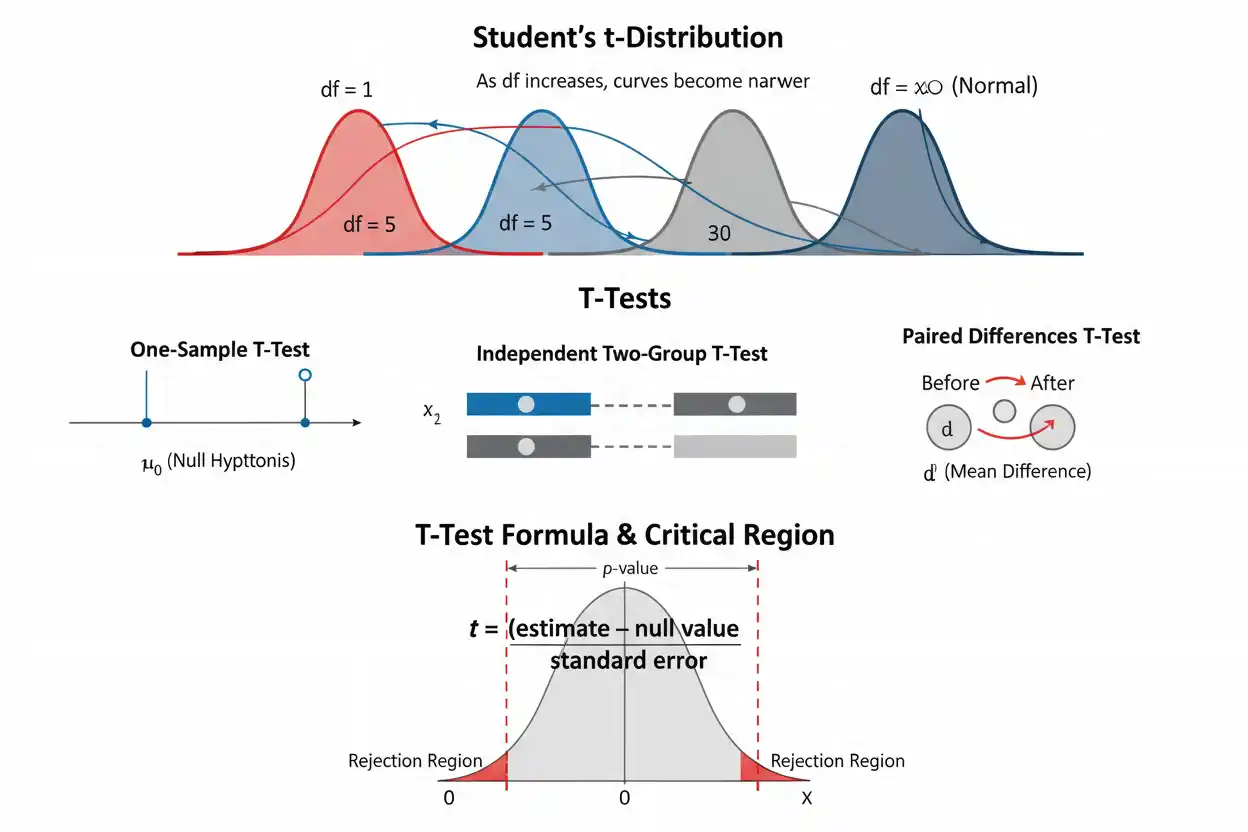
A t-test is a statistical hypothesis test used to evaluate whether a mean, a difference between means, or a mean paired difference is sufficiently large relative to its estimated sampling uncertainty to provide evidence against a specified null hypothesis. The defining feature of a t-test is that the relevant population standard deviation is unknown and is estimated from sample data, which introduces additional uncertainty and leads to a Student’s t reference distribution rather than an exact standard normal reference distribution under the classical normal-theory model. The one-sample t-test compares a sample mean with a hypothesized population mean, the independent-samples t-test compares means from separate groups, and the paired t-test analyzes the mean of within-pair differences when observations are naturally matched or repeatedly measured. In each case, the core logic is the same: subtract the null value from an estimated effect, divide by an appropriate standard error, and evaluate how extreme the resulting t statistic is under the null hypothesis. Correct interpretation requires more than checking whether a p-value falls below 0.05, because effect size, confidence intervals, sample size, independence, outliers, distribution shape, study design, and the practical importance of the estimated difference all affect what the result actually means.
The t-test sits within the inferential framework established by statistics basics and relies directly on the behavior of sampling distributions. Its denominator is built from estimated variability, making standard deviation and variance central to the calculation, while the relationship between t statistics and standardized normal quantities becomes especially clear when compared with the z-score.
What Is a t-Test?
A t-test asks whether an observed mean difference is large relative to the uncertainty expected from sampling variation. The result is summarized through a t statistic, which measures the estimated effect in units of its estimated standard error.
The generic form is:
t = (Estimate − Null value) / Standard error
A large positive t statistic indicates that the estimate lies many estimated standard errors above the null value, while a large negative t statistic indicates that it lies many estimated standard errors below the null value. A t statistic near zero indicates that the estimate is close to the null value relative to its uncertainty.
The t-test does not measure whether a result is “large” in practical units by itself. It measures how large the estimated difference is relative to the precision with which that difference has been estimated.
Why Is It Called a t-Test?
The t-test uses Student’s t distribution as its reference distribution under the classical model. The t distribution resembles the standard normal distribution but has heavier tails, reflecting the additional uncertainty created when the unknown population standard deviation is replaced with an estimate from sample data.
Its exact shape depends on:
degrees of freedom
As degrees of freedom increase, the t distribution becomes increasingly similar to:
N(0,1)
the standard normal distribution.
For very large degrees of freedom, the practical difference between corresponding t and z critical values becomes small.
For small samples, however, the heavier tails of the t distribution are important and produce larger critical values than the standard normal model.
General t-Test Formula
The basic structure of a t-test can be written as:
t = (Observed estimate − Hypothesized value) / Estimated standard error
Different t-tests use different estimates and standard errors.
For a one-sample t-test:
t = (x̄ − μ₀)/(s/√n)
For an independent two-sample Welch t-test:
t = [(x̄₁ − x̄₂) − Δ₀] / √(s₁²/n₁ + s₂²/n₂)
For a paired t-test:
t = (d̄ − μd,0)/(sd/√n)
Although these formulas look different, each standardizes a difference relative to its sampling uncertainty.
One-Sample t-Test
A one-sample t-test compares a sample mean with a specified population mean under the null hypothesis.
The hypotheses may be:
H₀: μ = μ₀
H₁: μ ≠ μ₀
for a two-sided test.
The test statistic is:
t = (x̄ − μ₀)/(s/√n)
where:
- x̄ = sample mean
- μ₀ = hypothesized population mean
- s = sample standard deviation
- n = sample size
Under the standard one-sample t-test model and H₀:
t ~ t₍ₙ₋₁₎
so:
df = n − 1
The denominator:
s/√n
is the estimated standard error of the sample mean.
One-Sample t-Test Example
Suppose a sample contains:
n = 25
observations with:
x̄ = 52
s = 10
and the null hypothesis is:
H₀: μ = 48
against:
H₁: μ ≠ 48
First calculate the estimated standard error:
SE = s/√n
SE = 10/√25
SE = 10/5
SE = 2
Now calculate the t statistic:
t = (52 − 48)/2
t = 4/2
t = 2
Degrees of freedom are:
df = 25 − 1
df = 24
The two-sided p-value for:
t = 2
with:
df = 24
is approximately:
p ≈ 0.057
Therefore, at:
α = 0.05
the result narrowly fails to reach the conventional 5% significance threshold.
The correct conclusion is:
fail to reject H₀ at α = 0.05
not:
prove that μ = 48.
Interpreting the One-Sample Result
The observed sample mean is:
4 units
above the hypothesized mean, and that difference equals:
2 estimated standard errors.
This provides some evidence against H₀, but under a two-sided t-test with 24 degrees of freedom it is not quite enough to cross a 0.05 decision threshold.
That distinction illustrates why a t-test should not be interpreted as a binary truth machine. A result with:
p ≈ 0.057
is not fundamentally different in evidential strength from a result with:
p ≈ 0.049.
The numerical estimate, confidence interval, p-value, sample size, and substantive importance should be interpreted together.
One-Sided t-Test
A one-sided t-test is appropriate when the alternative hypothesis is directional and that direction is specified before observing the result.
For an upper-tailed test:
H₀: μ = μ₀
H₁: μ > μ₀
the p-value is:
P(T ≥ t_obs)
under the null t distribution.
For a lower-tailed test:
H₁: μ < μ₀
the p-value is:
P(T ≤ t_obs)
The direction should arise from the research question rather than being selected after examining the sign of the observed difference.
Changing from a two-sided test to a one-sided t-test after seeing the data alters the intended false-positive properties of the procedure.
Two-Sided t-Test
A two-sided t-test is used when departures in either direction are relevant.
The alternative is:
H₁: μ ≠ μ₀
A sufficiently large positive or negative t statistic can lead to rejection.
For a symmetric t distribution, the two-sided p-value can be expressed as:
p = 2P(T ≥ |t_obs|)
where T follows the appropriate t distribution under H₀.
Two-sided testing is commonly appropriate when both increases and decreases would be scientifically meaningful or when direction was not justified in advance.
Degrees of Freedom
Degrees of freedom determine the exact shape of the t reference distribution.
For a one-sample t-test:
df = n − 1
The loss of one degree of freedom reflects the fact that the sample mean is estimated from the same data used to estimate variability.
With:
n = 5
we have:
df = 4
and the t distribution is noticeably heavier-tailed than a standard normal distribution.
With:
n = 1,000
we have:
df = 999
and the t distribution is extremely close to the standard normal distribution.
Thus, small samples require more extreme t statistics to cross the same conventional significance level.
t Distribution vs Normal Distribution
The t distribution and standard normal distribution are both symmetric around zero, but the t distribution allocates more probability to its tails.
For a two-sided 95% interval:
z* ≈ 1.960
For:
df = 4
the corresponding t critical value is approximately:
t* ≈ 2.776
For:
df = 24
it is approximately:
t* ≈ 2.064
For:
df = 100
it is approximately:
t* ≈ 1.984
As degrees of freedom grow, the t critical value approaches:
1.960
The heavier tails account for uncertainty introduced by estimating σ with s.
Why Estimating Standard Deviation Matters
If the population standard deviation σ were known, the standardized sample mean could be written:
z = (x̄ − μ₀)/(σ/√n)
Under normal sampling, this follows the standard normal distribution under H₀.
In a t-test, σ is unknown, so it is replaced by:
s
giving:
t = (x̄ − μ₀)/(s/√n)
The denominator is now random because s varies from sample to sample. That extra randomness makes the standardized statistic more variable than a z statistic would be if σ were truly known.
The t distribution accounts for this additional uncertainty.
Independent-Samples t-Test
An independent-samples t-test compares means from two groups whose observations are independent across groups.
Examples include comparing:
- Group A with Group B,
- treatment with control,
- one region with another,
provided the observational structure justifies treating the groups as independent.
The null hypothesis is often:
H₀: μ₁ − μ₂ = 0
More generally:
H₀: μ₁ − μ₂ = Δ₀
where Δ₀ is a specified difference.
There are two major versions of the independent t-test:
Welch t-test
and:
pooled equal-variance t-test.
Welch’s version is generally the safer default when equal population variances cannot be confidently assumed.
Welch t-Test Formula
The Welch t statistic is:
t = [(x̄₁ − x̄₂) − Δ₀] / √(s₁²/n₁ + s₂²/n₂)
where:
- x̄₁, x̄₂ = sample means
- s₁², s₂² = sample variances
- n₁, n₂ = sample sizes
- Δ₀ = hypothesized population mean difference
For the common null:
Δ₀ = 0
the formula becomes:
t = (x̄₁ − x̄₂) / √(s₁²/n₁ + s₂²/n₂)
Unlike the pooled t-test, Welch’s method does not require equal population variances.
Welch Degrees of Freedom
Welch’s approximate degrees of freedom are:
df ≈ (s₁²/n₁ + s₂²/n₂)² /
[(s₁²/n₁)²/(n₁−1) + (s₂²/n₂)²/(n₂−1)]
The result is often noninteger.
Statistical software commonly uses the decimal value directly when evaluating the t distribution.
This approximation reflects the fact that each group’s estimated variance contributes differently to the uncertainty of the mean difference.
When sample sizes and variances are equal, Welch’s result becomes similar to the pooled equal-variance t-test.
Welch t-Test Example
Suppose Group 1 has:
n₁ = 20
x̄₁ = 85
s₁ = 10
and Group 2 has:
n₂ = 30
x̄₂ = 78
s₂ = 12
Test:
H₀: μ₁ − μ₂ = 0
against:
H₁: μ₁ − μ₂ ≠ 0
The observed mean difference is:
85 − 78 = 7
Calculate the standard error:
SE = √(10²/20 + 12²/30)
= √(100/20 + 144/30)
= √(5 + 4.8)
= √9.8
≈ 3.130
Therefore:
t = 7/3.130
t ≈ 2.236
Now calculate the approximate degrees of freedom:
df ≈ 44.0
after rounding.
The two-sided p-value is approximately:
p ≈ 0.030
Therefore, at:
α = 0.05
the data provide evidence against equal population means under the Welch t-test assumptions.
Interpreting the Welch Example
The estimated mean difference is:
7 units
and its estimated standard error is approximately:
3.13 units.
Therefore, the observed difference is approximately:
2.24 standard errors
away from the null difference of zero.
The statistical result indicates that a difference at least this extreme would be relatively unusual under H₀ and the Welch model. It does not establish that group membership caused the mean difference, because causation depends on how the groups were formed and how the study was designed.
The magnitude:
7 units
should therefore be interpreted separately from its statistical significance.
Equal-Variance Pooled t-Test
The pooled two-sample t-test assumes that the two population variances are equal:
σ₁² = σ₂² = σ²
Under this assumption, the two sample variances can be combined into a pooled variance estimator:
sₚ² = [(n₁−1)s₁² + (n₂−1)s₂²]/(n₁+n₂−2)
Then:
sₚ = √sₚ²
The pooled t statistic is:
t = [(x̄₁−x̄₂) − Δ₀] /
[sₚ√(1/n₁ + 1/n₂)]
with:
df = n₁ + n₂ − 2
The pooled t-test can be efficient when the equal-variance assumption is justified, but Welch’s t-test avoids depending on that assumption.
Pooled t-Test Example
Suppose:
n₁ = 15
x̄₁ = 24
s₁ = 4
and:
n₂ = 15
x̄₂ = 20
s₂ = 4
The variances are identical in the sample, and suppose the equal-population-variance model is substantively justified.
Pooled variance is:
sₚ² = [(14)(16) + (14)(16)]/(15+15−2)
= 448/28
= 16
Therefore:
sₚ = 4
The standard error of the mean difference is:
SE = 4√(1/15 + 1/15)
= 4√(2/15)
≈ 1.461
The t statistic is:
t = (24 − 20)/1.461
t ≈ 2.738
Degrees of freedom:
df = 28
The corresponding two-sided p-value is approximately:
p ≈ 0.011
This indicates evidence against equal means under the pooled-model assumptions.
Welch vs Pooled t-Test
The main difference is the variance assumption.
Welch’s t-test allows:
σ₁² ≠ σ₂²
and uses separate variance estimates.
The pooled t-test assumes:
σ₁² = σ₂²
and combines them into a common variance estimate.
If variances and group sizes are similar, the results may be almost identical. If group variances differ substantially—especially when sample sizes are unequal—the pooled test can produce misleading standard errors and Type I error behavior.
Because Welch’s t-test performs well in many equal-variance settings while providing protection against unequal variances, it is often preferred unless there is a substantive reason to use the pooled formulation.
Should You Test Variances First?
A common strategy is to perform a variance-equality test and then choose between pooled and Welch t-tests based on whether that preliminary test is significant.
This two-stage strategy can create unnecessary complications because the variance test itself is uncertain and can alter the overall operating characteristics of the analysis.
A simpler approach is often to use Welch’s t-test directly when equal population variances are not a core modeling assumption.
If equal variance is scientifically justified by design or process knowledge, the pooled model can still be appropriate.
The choice should be based on the intended model rather than a mechanical preliminary significance test alone.
Paired t-Test
A paired t-test is used when observations come in meaningful pairs.
Examples include:
- measurements before and after an intervention on the same individuals,
- matched experimental units,
- left and right measurements from the same subject,
- deliberately matched case-control pairs.
The analysis does not treat the two measurement columns as independent groups. Instead, it computes one difference within each pair:
dᵢ = xᵢ − yᵢ
and then performs a one-sample t-test on those differences.
The pairing matters because within-pair correlation can reduce irrelevant between-unit variability and improve precision when the matching is meaningful.
Paired t-Test Formula
Let:
d₁, d₂, …, dₙ
be the paired differences.
Calculate:
d̄ = Σdᵢ/n
and their sample standard deviation:
sd
The paired t statistic is:
t = (d̄ − μd,0)/(sd/√n)
For the common null hypothesis:
H₀: μd = 0
this becomes:
t = d̄/(sd/√n)
Degrees of freedom are:
df = n − 1
The paired t-test therefore has exactly the same mathematical structure as a one-sample t-test, with the differences serving as the observed variable.
Paired t-Test Example
Suppose six units are measured before and after a change.
| Unit | Before | After | Difference: After − Before |
|---|---|---|---|
| 1 | 10 | 12 | 2 |
| 2 | 13 | 16 | 3 |
| 3 | 15 | 16 | 1 |
| 4 | 12 | 14 | 2 |
| 5 | 18 | 21 | 3 |
| 6 | 14 | 15 | 1 |
The differences are:
2, 3, 1, 2, 3, 1
Their mean is:
d̄ = 12/6
d̄ = 2
The deviations from 2 are:
0, 1, −1, 0, 1, −1
Their squared deviations sum to:
4
Therefore:
sd² = 4/(6 − 1)
sd² = 0.8
and:
sd ≈ 0.8944
The standard error is:
SE = 0.8944/√6
≈ 0.3651
Thus:
t = 2/0.3651
t ≈ 5.478
with:
df = 5
The two-sided p-value is approximately:
p ≈ 0.0028
The paired data therefore provide strong evidence of a nonzero mean change under the t-test model.
Why Pairing Can Increase Precision
Suppose individuals differ substantially from one another in their baseline levels, but each person’s repeated measurements are strongly correlated. An independent-groups analysis would allow those large between-person differences to contribute to the error variability.
The paired t-test removes each unit’s baseline level by working with:
within-unit differences.
If those differences have relatively small standard deviation, the estimated mean change can be much more precise.
Pairing is beneficial when the pairs are genuinely linked.
Arbitrarily pairing unrelated observations does not create legitimate precision and can invalidate the analysis.
Paired vs Independent t-Test
Use a paired t-test when the observations are linked one-to-one in a meaningful way.
Use an independent-samples t-test when observations in one group are independent of observations in the other group.
For example:
before and after on the same 30 people
is paired.
By contrast:
30 people receiving Treatment A and a separate 30 people receiving Treatment B
is independent unless the participants were deliberately matched and the analysis preserves those matched pairs.
Choosing the wrong dependence structure changes the standard error and therefore changes the t statistic, confidence interval, and p-value.
t-Test Assumptions
The exact assumptions depend on which t-test is used, but several principles recur. Observations should arise from a design that justifies the intended inferential target, and the independence or pairing structure must be correctly represented.
For a one-sample t-test, observations are ordinarily assumed independent and identically distributed around a common population mean. For a paired t-test, the pair differences are the independent observational units. For an independent two-sample t-test, observations should be independent within and across groups unless a more complex dependence structure is modeled.
Normality is most important for exact small-sample t distribution results. With larger samples, the mean-based procedures can often remain useful under broader distribution shapes because of sampling-distribution approximations, but extreme skewness, heavy tails, severe outliers, or dependence can still cause substantial problems.
Independence Is More Important Than Many Analysts Realize
A t-test can tolerate moderate non-normality much better than it can tolerate incorrectly treated dependence.
Suppose one individual contributes ten repeated measurements. Counting those measurements as ten independent people can make the effective sample size appear much larger than it really is.
Similarly, observations collected from members of the same cluster can share common influences.
The usual t-test standard errors assume the relevant units of analysis have the dependence structure specified by the test.
If that structure is wrong, a perfectly calculated formula can yield misleading uncertainty.
Normality Assumption
For an exact one-sample t-test with small n, the data are commonly modeled as independent observations from a normal population.
For a paired t-test, the relevant normality assumption concerns:
the distribution of paired differences
rather than the separate before and after measurement distributions.
For independent-group t-tests, normality concerns the distributions of observations or errors within the groups under the classical model.
The t-test is often reasonably robust to moderate deviations from normality when samples are not tiny and distributions are not dominated by extreme tails, but there is no universal sample-size threshold at which all departures become irrelevant.
Outliers and the t-Test
The t-test is based on means and standard deviations, both of which are sensitive to extreme observations.
An outlier can:
- move the sample mean,
- increase the sample standard deviation,
- alter the t statistic,
- change the confidence interval,
- potentially reverse the conclusion.
An unusual value should therefore be investigated rather than automatically deleted.
If the observation is valid, its influence may represent real population behavior.
If it is a confirmed measurement or data-entry error, correction or justified exclusion may be appropriate.
Sensitivity analysis can help show whether conclusions depend heavily on individual observations.
Equal Variance Assumption
The ordinary pooled independent t-test assumes:
σ₁² = σ₂²
Welch’s t-test does not.
This distinction does not arise in the same way for a one-sample or paired t-test because there is only one variable being analyzed in those formulations—the original observations or the paired differences.
When independent groups have substantially different variances and sample sizes are also unequal, Welch’s approach is especially valuable because it adjusts both the standard error and degrees of freedom.
t-Test and Sample Size
Sample size influences the t-test in several ways. Larger samples generally reduce standard errors, provide more degrees of freedom, make the t distribution closer to normal, and increase statistical power for a fixed true effect.
For a one-sample t-test:
SE = s/√n
If the estimated standard deviation remains similar and sample size increases by a factor of four, the standard error is approximately halved.
That makes a fixed mean difference twice as large in standard-error units.
However, a larger sample does not correct biased sampling, invalid measurements, or a wrong dependence model.
t-Test and Statistical Power
Power is the probability of rejecting H₀ when a specified alternative is true.
For a t-test, power generally increases with:
- larger sample size,
- larger true mean difference,
- smaller population variability,
- a larger significance threshold,
- efficient design.
A study can produce:
p > 0.05
because the true effect is near zero, but it can also produce the same result because the sample is too small or noisy to estimate the effect precisely.
Therefore, failing to reject the null hypothesis does not prove that the underlying means are identical.
t-Test and Effect Size
Statistical significance depends partly on sample size, so effect size should be considered separately.
For a one-sample setting, a standardized effect can be expressed as:
d = (x̄ − μ₀)/s
For two independent groups under an appropriate pooled-standard-deviation convention:
d = (x̄₁ − x̄₂)/sₚ
These standardized effects express the mean difference relative to a standard deviation scale.
However, practical interpretation should still consider the original units. A standardized effect can aid comparison, but a difference of 5 units may be important in one application and negligible in another.
Relationship Between t and Standardized Effect Size
For a one-sample t-test:
t = (x̄ − μ₀)/(s/√n)
and:
d = (x̄ − μ₀)/s
Therefore:
t = d√n
This relationship shows explicitly how statistical significance depends on both standardized effect size and sample size.
For a fixed d, increasing n increases |t|.
Thus, a very small effect can become statistically significant in a sufficiently large sample, while a substantial effect can remain statistically uncertain in a very small sample.
Confidence Interval for a One-Sample Mean
A two-sided confidence interval for μ is:
x̄ ± t* s/√n
where:
t*
is the critical value from the t distribution with:
df = n − 1
Suppose:
x̄ = 52
s = 10
n = 25
For 95% confidence:
t* ≈ 2.064
because:
df = 24
The margin of error is:
2.064(10/5)
= 2.064(2)
= 4.128
Therefore:
95% CI ≈ 52 ± 4.128
or:
(47.87, 56.13)
The null value 48 lies inside this interval, which is consistent with the corresponding two-sided t-test failing to reject at α = 0.05.
Confidence Interval and t-Test Equivalence
For many standard two-sided t procedures, the confidence interval and hypothesis test are mathematically linked.
If a:
95% confidence interval
for a parameter excludes the null value, the corresponding two-sided test at:
α = 0.05
rejects H₀.
If the interval includes the null value, the test fails to reject.
This equivalence assumes the interval and test use the same statistical model and standard-error method.
The confidence interval often communicates more information because it displays both the estimated effect and its uncertainty rather than only a significance classification.
Confidence Interval for a Difference Between Means
Under Welch’s two-sample method, an interval for:
μ₁ − μ₂
takes the form:
(x̄₁ − x̄₂) ± t*√(s₁²/n₁ + s₂²/n₂)
where t* uses the Welch degrees of freedom.
For the earlier example:
Difference = 7
SE ≈ 3.130
df ≈ 44
A 95% critical value is approximately:
t* ≈ 2.015
Therefore:
Margin ≈ 2.015(3.130)
≈ 6.307
The interval is approximately:
7 ± 6.307
or:
(0.69, 13.31)
This interval excludes zero but also shows considerable uncertainty about the true magnitude of the population mean difference.
Confidence Interval for Paired Differences
For paired data, the confidence interval is constructed for the population mean difference:
μd
using:
d̄ ± t* sd/√n
For the earlier paired example:
d̄ = 2
sd ≈ 0.8944
n = 6
df = 5
The 95% critical value is approximately:
t* ≈ 2.571
The margin is:
2.571(0.3651)
≈ 0.939
Therefore:
95% CI ≈ 2 ± 0.939
or:
(1.06, 2.94)
The interval indicates that the population mean paired increase is estimated to be positive and roughly between 1.06 and 2.94 units under the model.
t-Test and Sampling Distributions
The logic of every t-test comes from sampling distributions. If repeated samples were drawn under the null hypothesis, the estimated mean difference and standard error would vary from sample to sample, producing a distribution of t statistics.
Under the classical one-sample normal model:
T = (X̄ − μ)/(S/√n)
follows a Student’s t distribution with:
n − 1
degrees of freedom.
The p-value is calculated from the location of the observed t statistic within that null sampling distribution.
Thus, the test is fundamentally a repeated-sampling probability argument.
t-Test and Standard Deviation
The standard deviation directly controls the denominator of the t statistic.
For a one-sample t-test:
t = (x̄ − μ₀)/(s/√n)
If s becomes larger while the mean difference and n remain fixed, the denominator increases and |t| decreases.
Therefore, highly variable observations provide less precise information about a mean than tightly clustered observations.
The same principle applies to two-sample and paired tests: greater unexplained variability produces larger standard errors and generally weaker evidence for a fixed raw mean difference.
t-Test and Variance
Because:
s = √s²
the t-test can equally be understood in terms of estimated variance.
For Welch’s test:
SE² = s₁²/n₁ + s₂²/n₂
The variance contributions add because the two sample means are independent under the model.
The standard error is the square root of this sampling variance.
This illustrates a broader statistical principle: independent variances add naturally, while standard deviations do not simply add.
t-Test vs z-Test
A t-test is generally used for mean inference when the relevant population standard deviation is unknown and estimated from sample data.
A z-test for a mean can be appropriate when:
σ
is genuinely known or when a specific asymptotic procedure has a standard normal reference distribution.
The one-sample formulas resemble one another:
z = (x̄ − μ₀)/(σ/√n)
t = (x̄ − μ₀)/(s/√n)
The difference between σ and s matters because s is random.
When degrees of freedom become large, the t and standard normal distributions become very similar, so numerical results can converge.
t-Test and z-Score
A z-score usually measures standardized distance using a known or specified mean and standard deviation:
z = (x − μ)/σ
A t statistic also measures standardized distance, but its denominator typically contains an estimated standard error derived from sample variability.
Thus:
z-score → often standardized observation or known-σ statistic
t statistic → estimated effect relative to an estimated standard error
They share the logic of standardization but use different reference distributions and statistical contexts.
t-Test vs ANOVA
A t-test is naturally suited to one mean or a comparison between two means.
When three or more group means are compared simultaneously, analysis of variance provides a framework for testing whether all population means are equal without performing a large collection of unadjusted pairwise t-tests.
For exactly two independent groups under compatible assumptions, the ordinary pooled two-sample t-test and one-way ANOVA produce equivalent significance results because:
F = t²
for that two-group comparison.
The broader ANOVA framework becomes more useful as the number of groups or model terms increases.
Multiple t-Tests
Suppose ten group comparisons are each tested at:
α = 0.05
Running ten independent tests without adjustment creates more opportunities for at least one false rejection than running only one test.
If all ten null hypotheses are true and the tests are independent, the probability of at least one false-positive rejection is:
1 − (1 − 0.05)¹⁰
= 1 − 0.95¹⁰
≈ 0.401
or about:
40.1%
The exact behavior differs when tests are dependent, but the broader issue remains: repeated testing changes the false-positive environment.
Multiple-comparison procedures may therefore be needed when many t-tests are performed as part of one analytical family.
p-Value Interpretation
Suppose a t-test produces:
p = 0.03
A correct interpretation is that, under H₀ and the assumptions of the test, a t statistic at least as extreme as the observed statistic would occur with probability about 3% according to the relevant tail definition.
It is incorrect to say:
“There is a 3% probability the null hypothesis is true.”
It is also generally incorrect to say:
“There is a 97% probability the alternative is true.”
A frequentist t-test conditions on H₀ and evaluates data extremeness. It does not directly calculate posterior probabilities of hypotheses.
Failing to Reject H₀
Suppose:
p = 0.30
The proper statistical decision at α = 0.05 is:
fail to reject H₀.
This does not establish:
μ₁ = μ₂
or:
μ = μ₀
as exact truths.
The data may simply be too imprecise to distinguish the observed effect from sampling variation.
If demonstrating that two means are sufficiently similar is the actual objective, an equivalence or noninferiority framework may be more appropriate than interpreting a non-significant ordinary t-test as proof of equality.
Statistical Significance vs Practical Significance
Suppose a study with:
n = 100,000
detects a mean difference of:
0.05 units
with:
p < 0.001.
The t-test result is statistically significant.
If a difference smaller than:
2 units
has no practical consequence, the effect may be operationally unimportant despite the tiny p-value.
Conversely, a small study might estimate a 5-unit difference with a wide confidence interval and:
p = 0.08.
That result may still deserve substantive attention because the estimated magnitude is potentially important but uncertain.
Effect size and uncertainty should therefore accompany significance testing.
Statistical Significance Does Not Prove Causation
A t-test can detect a mean difference between two observed groups, but it does not identify why the difference exists.
If the groups were created by random assignment in a well-designed experiment, a causal interpretation can be much more defensible.
If the groups arose observationally, the mean difference could reflect:
- confounding,
- selection,
- reverse causation,
- measurement differences,
- other group characteristics.
The t-test evaluates an inferential comparison of means. Study design determines whether that comparison can be interpreted causally.
Missing Data and the t-Test
Missing observations can affect both the sample size and the composition of the analyzed sample.
In a paired t-test, a pair generally requires both measurements to calculate:
dᵢ
so missing one member of a pair can remove that pair from a simple complete-pair analysis.
If missingness is systematically related to outcomes or treatment response, simply deleting incomplete observations can introduce bias.
A larger remaining n does not solve that problem.
The missing-data mechanism should therefore be considered independently of the t-test formula.
Small Samples
A t-test was specifically developed to handle uncertainty from estimating population variability in relatively small samples, but this does not mean every tiny sample is adequate for meaningful inference.
With:
n = 4
a one-sample test has:
df = 3
and both the estimate of s and the mean can be highly sensitive to individual observations.
The exact t distribution protects the nominal test under the classical normal model, but the small sample provides little ability to diagnose whether that model is plausible.
Small-sample t-tests therefore require especially careful attention to data quality, outliers, study design, and distribution shape.
Large Samples
As n grows, t critical values approach z critical values, and sample means often have approximately normal sampling distributions under broad conditions.
However, large samples create a different interpretive issue: even tiny departures from the null can produce large t statistics because standard errors become very small.
For example, if:
Difference = 0.1
but:
SE = 0.01
then:
t = 10
which produces an extremely small p-value.
The result may be statistically decisive while the raw effect remains substantively minor.
Large n improves precision; it does not determine importance.
Nonparametric Alternatives
When mean-based t-test assumptions are poorly aligned with the scientific question or data structure, rank-based or resampling methods can sometimes provide alternatives.
However, such methods do not necessarily test exactly the same hypothesis as a t-test. A rank-based test should not automatically be described as a “t-test without normality” because its parameter interpretation and assumptions can differ.
Similarly, bootstrap or permutation procedures require their own conditions.
The method should be selected according to the target estimand, sampling design, distributional structure, and robustness requirements rather than simply replacing one test whenever a normality diagnostic looks imperfect.
Transformations Before a t-Test
A transformation can sometimes make a mean comparison more scientifically meaningful or stabilize variability.
For positive skewed data, one might analyze:
ln(X)
rather than X.
The resulting t-test concerns the mean on the transformed scale.
That changes interpretation.
For example, differences between mean logarithms can correspond to ratios of geometric means after back-transformation under suitable conditions.
A transformation should therefore be selected for substantive and model-based reasons, not merely to force a desired p-value.
Reporting a t-Test
A useful t-test report includes more than:
significant
or:
not significant.
For a one-sample test, a clear report might state:
“The sample mean was 52.0 compared with a null mean of 48.0, t(24) = 2.00, p = 0.057, with a 95% confidence interval for μ of approximately 47.87 to 56.13.”
For an independent-group comparison, report:
- both group means,
- relevant standard deviations,
- estimated mean difference,
- confidence interval,
- test statistic,
- degrees of freedom,
- p-value,
- whether Welch or pooled variance estimation was used.
For paired data, report the mean and standard deviation of the paired differences.
This makes the statistical result interpretable rather than reducing the analysis to a threshold.
Common t-Test Mistakes
A common mistake is using an independent t-test for paired measurements such as before-and-after observations from the same individuals. The dependence should instead be represented by analyzing within-pair differences.
Another error is automatically using a pooled t-test without considering whether equal population variances are a justified model assumption. Welch’s t-test is often more appropriate when variance equality is uncertain.
A third mistake is choosing a one-sided alternative after observing the data. Direction should be specified from the research question before the result is known.
Analysts also sometimes interpret p > 0.05 as proof that two population means are equal, even though a non-significant result can arise from low precision or low power.
Another common error is treating a small p-value as proof of a large or important effect.
Outliers, dependence, clustering, nonrepresentative sampling, and missing-data mechanisms can also invalidate a superficially correct t-test.
Finally, the population parameter, effect estimate, confidence interval, and study design should not be replaced by a binary significant/not-significant label.
How to Perform a t-Test Step by Step
Begin by identifying the parameter of interest and the data structure. If one sample mean is being compared with a benchmark, use a one-sample framework. If two separate groups are being compared, use an independent-samples framework, usually Welch’s method unless equal variances are substantively justified. If observations are matched or repeatedly measured, calculate the within-pair differences and use a paired t-test.
Next state the null and alternative hypotheses before examining the inferential result, determine whether the test is one-sided or two-sided, calculate the relevant estimate and standard error, and then form:
t = (Estimate − Null value)/SE
Determine the correct degrees of freedom and obtain the p-value from the corresponding t distribution. Construct a confidence interval for the same effect, examine the estimated magnitude in practical units, and check whether outliers, dependence, distribution shape, missing data, or study design create reasons for caution.
The final interpretation should answer the original question in terms of both evidence and effect size.
Full One-Sample t-Test Worked Example
Suppose a process is believed to have population mean:
μ₀ = 100
A random sample of:
n = 16
independent observations gives:
x̄ = 106
s = 8
Test:
H₀: μ = 100
against:
H₁: μ ≠ 100
Step 1: Calculate Standard Error
SE = s/√n
= 8/√16
= 8/4
= 2
Step 2: Calculate t
t = (106 − 100)/2
t = 3
Step 3: Degrees of Freedom
df = 16 − 1
df = 15
Step 4: Calculate the p-Value
For:
t = 3
with:
df = 15
the two-sided p-value is approximately:
p ≈ 0.009
Step 5: Decision
At:
α = 0.05
we have:
p < 0.05
so:
reject H₀
under the t-test procedure.
Step 6: Confidence Interval
For 95% confidence with:
df = 15
the critical value is approximately:
t* = 2.131
The margin is:
2.131(2)
= 4.262
Therefore:
95% CI ≈ 106 ± 4.262
or:
(101.74, 110.26)
The null value 100 falls outside this interval, matching the two-sided test conclusion.
Full Welch t-Test Worked Example
Suppose:
Group 1: n₁ = 40, x̄₁ = 72, s₁ = 10
Group 2: n₂ = 30, x̄₂ = 65, s₂ = 15
Test:
H₀: μ₁ − μ₂ = 0
The mean difference is:
72 − 65 = 7
Standard error:
SE = √(10²/40 + 15²/30)
= √(100/40 + 225/30)
= √(2.5 + 7.5)
= √10
≈ 3.162
Therefore:
t = 7/3.162
≈ 2.214
Welch degrees of freedom are approximately:
df ≈ 45.6
The corresponding two-sided p-value is approximately:
p ≈ 0.032
Therefore, at the 5% level, the test provides evidence of a difference in population means under the Welch model.
The estimated mean difference remains:
7 units
which should be interpreted in the original measurement context rather than replaced by the significance label.
Full Paired t-Test Worked Example
Suppose paired differences are:
3, 1, 4, 2, 2, 3, 1, 4
There are:
n = 8
pairs.
The mean difference is:
d̄ = 20/8
d̄ = 2.5
The squared deviations from 2.5 sum to:
10
Therefore:
sd² = 10/(8 − 1)
= 10/7
≈ 1.4286
and:
sd ≈ 1.195
The standard error is:
SE = 1.195/√8
≈ 0.4226
The t statistic is:
t = 2.5/0.4226
≈ 5.916
Degrees of freedom:
df = 7
This produces a very small two-sided p-value, providing strong evidence that the population mean paired difference is not zero under the model.
The effect estimate itself remains:
2.5 units
and should be reported along with its confidence interval and substantive interpretation.
Frequently Asked Questions About the t-Test
What is a t-test?
A t-test is a hypothesis test for a mean or mean difference that standardizes the estimated effect by an estimated standard error and uses a Student’s t reference distribution.
What is the basic t-test formula?
The general structure is:
t = (Estimate − Null value)/Standard error
What is the one-sample t-test formula?
t = (x̄ − μ₀)/(s/√n)
What are the degrees of freedom for a one-sample t-test?
df = n − 1
What does a t statistic mean?
It measures how many estimated standard errors the observed estimate lies from the null value.
What does t = 0 mean?
The observed estimate equals the null value exactly.
Can a t statistic be negative?
Yes. A negative value means the estimate lies below the null value according to the direction used in the calculation.
Does a negative t statistic mean the result is insignificant?
No. Statistical extremeness depends on the magnitude and direction relative to the stated alternative. A large negative t can be highly significant.
Why does a t-test use the t distribution?
Because the population standard deviation is unknown and estimated from sample data, creating additional uncertainty that the t distribution represents under the classical model.
What happens as degrees of freedom increase?
The t distribution approaches the standard normal distribution.
What is a one-sample t-test used for?
It compares a sample mean with a hypothesized population mean.
What is an independent-samples t-test?
It compares population means using observations from separate independent groups.
What is Welch’s t-test?
Welch’s t-test compares two independent means without assuming equal population variances.
What is a pooled t-test?
It compares two independent means under an equal-population-variance assumption and uses a pooled variance estimate.
Which is better: Welch or pooled t-test?
Welch’s test is generally safer when equal population variances are uncertain. The pooled test is appropriate when the equal-variance model is substantively justified.
What is a paired t-test?
A paired t-test performs a one-sample t-test on within-pair differences from matched or repeated observations.
What are the degrees of freedom for a paired t-test?
With n paired differences:
df = n − 1
Is before-and-after data paired?
Yes, when the same observational units are measured at both times.
Can I use an independent t-test for paired data?
Ordinarily no. Doing so ignores the within-pair dependence and uses the wrong standard-error structure.
What assumptions does a t-test make?
The assumptions depend on the version, but the sampling or experimental design must support the target inference, dependence must be correctly represented, and classical exact small-sample procedures generally use an appropriate normal model for the observations or paired differences.
Must raw data be perfectly normal?
No. Moderate deviations can often be tolerated, particularly with adequate sample sizes, but severe skewness, heavy tails, or influential observations can still matter.
What distribution should be normal for a paired t-test?
The distribution of the paired differences is the relevant quantity under the classical normal model.
Does Welch’s t-test require equal variances?
No.
Does the pooled t-test require equal variances?
Yes, as part of its classical model.
What is the standard error in a one-sample t-test?
SE = s/√n
How does sample size affect a t-test?
Larger n generally reduces standard error, increases degrees of freedom, and increases power for a fixed true effect.
Does a large sample guarantee a valid t-test?
No. Large n does not correct dependence, biased sampling, invalid measurements, or a badly chosen model.
How do outliers affect a t-test?
They can strongly affect both the mean and standard deviation, thereby changing the t statistic and confidence interval.
What does p < 0.05 mean in a t-test?
It means the observed t statistic is sufficiently extreme under the null model to cross a preselected 0.05 significance threshold.
Does p < 0.05 mean H₀ has less than a 5% probability of being true?
No.
What does p > 0.05 mean?
It means the test fails to reject H₀ at the 0.05 level. It does not prove H₀.
Does a statistically significant t-test mean the effect is important?
Not necessarily. Effect size and practical relevance must be evaluated separately.
Can a tiny effect be statistically significant?
Yes. A sufficiently large sample can make a very small effect statistically detectable.
Can a large effect be non-significant?
Yes. A small or highly variable sample can estimate a substantial effect imprecisely.
What is the relationship between a t-test and a confidence interval?
For compatible two-sided procedures, rejecting H₀ at α = 0.05 corresponds to the null value lying outside the associated 95% confidence interval.
What is the difference between t and z?
A t statistic generally uses an estimated standard deviation and a t reference distribution, while a z statistic uses a known or asymptotically specified standard error with a standard normal reference distribution.
Is a t-test causal?
No. A t-test compares means. Causal interpretation depends on study design and identification assumptions.
What is the main rule when using a t-test?
Choose the version that matches the data structure, calculate the effect relative to the correct standard error, verify that the sampling assumptions are credible, and interpret the estimated difference and confidence interval alongside the p-value rather than treating statistical significance as the entire conclusion.




