


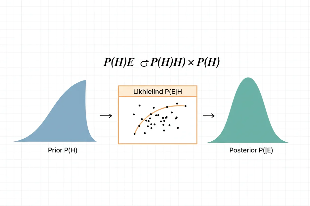
Bayes’ theorem is a probability rule for updating the probability of an event or hypothesis after new evidence is observed. It connects a probability in one conditional direction, such as P(B|A), with the reversed conditional probability P(A|B). The theorem is especially important when an observation is strongly associated with an event but the event itself is uncommon, because the underlying base rate can substantially change the final probability. Bayes’ theorem combines the prior probability of an event with the likelihood of observing the evidence under that event. The result is a posterior probability that reflects both the prior information and the new evidence. The theorem itself is an exact consequence of conditional probability rather than a rule that depends on statistical significance. Its correct use requires careful attention to the events being conditioned on, the denominator representing the total probability of the evidence, and the distinction between P(A|B) and P(B|A).
Within core statistics, Bayes’ theorem provides a foundation for conditional-probability reasoning, while the wider Statistics & Probability framework includes sampling, distributions, estimation, and hypothesis testing.
What Is Bayes’ Theorem?
Bayes’ theorem calculates the conditional probability of event A given that event B has occurred.
The basic formula is:
P(A|B) = P(B|A)P(A)/P(B)
where P(B) > 0.
Each term has a specific meaning:
- P(A|B) is the probability of A after observing B.
- P(B|A) is the probability of observing B if A is true.
- P(A) is the prior probability of A.
- P(B) is the overall probability of observing B.
In Bayesian terminology, P(A) is often called the prior, P(B|A) the likelihood, and P(A|B) the posterior. The denominator P(B) normalizes the result so that the posterior is a valid probability.
The theorem is simple algebraically, but most mistakes occur because conditional probabilities are interpreted in the wrong direction or because the overall probability P(B) is calculated incorrectly.
Bayes’ Theorem Formula
The standard form is:
P(A|B) = P(B|A)P(A)/P(B)
For two complementary possibilities, A and Aᶜ, the denominator can be expanded with the law of total probability:
P(B) = P(B|A)P(A) + P(B|Aᶜ)P(Aᶜ)
Therefore:
P(A|B) = P(B|A)P(A) / [P(B|A)P(A) + P(B|Aᶜ)P(Aᶜ)]
This expanded version is particularly useful for screening, classification, detection, and diagnostic-style problems in which an event can occur under either of two underlying states.
Because:
P(Aᶜ) = 1 − P(A)
the calculation can often be completed from a prior probability, a true-positive likelihood, and a false-positive likelihood.
Where Bayes’ Theorem Comes From
Bayes’ theorem follows directly from the definition of conditional probability.
For events A and B:
P(A|B) = P(A ∩ B)/P(B)
and:
P(B|A) = P(A ∩ B)/P(A)
Rearranging the second equation gives:
P(A ∩ B) = P(B|A)P(A)
Substituting that expression into the first equation produces:
P(A|B) = P(B|A)P(A)/P(B)
Thus, Bayes’ theorem is not an approximation. When the probabilities in the formula are correctly specified, the relationship is exact.
Understanding Prior, Likelihood, and Posterior
The easiest way to interpret Bayes’ theorem is as a sequence.
You begin with a prior probability:
P(A)
Then evidence B is observed. You ask how compatible that evidence is with A:
P(B|A)
However, observing B is meaningful only relative to how often B occurs overall. That role is handled by:
P(B)
The final updated probability is:
P(A|B)
The posterior can increase, decrease, or remain equal to the prior depending on how strongly the evidence favors A relative to competing possibilities.
If B is much more likely when A is true than when A is false, observing B will generally increase the probability of A. If B is equally likely whether A is true or false, then B provides no information about A.
Bayes’ Theorem Example
Suppose a manufacturing process produces defective items with probability 0.02.
A screening system flags 90% of defective items:
P(+|D) = 0.90
It also incorrectly flags 5% of nondefective items:
P(+|Dᶜ) = 0.05
The prior probability of a defective item is:
P(D) = 0.02
Therefore:
P(Dᶜ) = 1 − 0.02 = 0.98
The question is:
If an item is flagged, what is the probability that it is actually defective?
We want:
P(D|+)
Step 1: Calculate the Probability of a True Positive
The probability that an item is defective and flagged is:
P(+|D)P(D) = 0.90 × 0.02
= 0.018
Step 2: Calculate the Probability of a False Positive
The probability that an item is nondefective but still flagged is:
P(+|Dᶜ)P(Dᶜ) = 0.05 × 0.98
= 0.049
Step 3: Calculate the Overall Probability of a Positive Flag
P(+) = 0.018 + 0.049
P(+) = 0.067
Step 4: Apply Bayes’ Theorem
P(D|+) = 0.018/0.067
P(D|+) ≈ 0.2687
Therefore:
P(D|+) ≈ 26.87%
Even though the screening system detects 90% of defective items, a flagged item has only about a 26.87% probability of actually being defective under these assumptions.
The reason is the low 2% base rate. Nondefective items are so much more common that a 5% false-positive rate generates many false flags relative to the number of true positives.
The Same Example Using Frequencies
The same Bayes’ theorem calculation can be easier to understand by imagining 10,000 items.
With a 2% defect rate:
Defective items = 10,000 × 0.02 = 200
Nondefective items = 10,000 − 200 = 9,800
If 90% of defective items are flagged:
True positives = 200 × 0.90 = 180
If 5% of nondefective items are falsely flagged:
False positives = 9,800 × 0.05 = 490
The total number of positive flags is:
180 + 490 = 670
Among those 670 positive flags, 180 correspond to actual defects.
Therefore:
P(D|+) = 180/670
P(D|+) ≈ 0.2687
P(D|+) ≈ 26.87%
The frequency method and the probability formula produce the same result.
Why Base Rates Matter in Bayes’ Theorem
A common reasoning error is to focus only on P(B|A) and ignore P(A).
In the screening example, P(+|D) = 0.90 may sound like overwhelming evidence. However, the defect itself occurs only 2% of the time.
Bayes’ theorem combines both pieces of information. A highly informative signal can still produce a moderate posterior probability if the target event is sufficiently rare and false positives occur often enough.
This is known as the base-rate effect. Ignoring it can lead to serious overestimation of the probability that an underlying event is present after observing a positive signal.
P(A|B) Is Not the Same as P(B|A)
This distinction is fundamental.
Suppose:
P(+|D) = 0.90
That means 90% of defective items are expected to receive a positive flag.
It does not mean:
P(D|+) = 0.90
The second quantity asks what fraction of all positively flagged items are actually defective. It depends not only on the detection rate but also on the prior defect rate and the false-positive rate.
Bayes’ theorem is precisely the tool that connects these two conditional directions.
Bayes’ Theorem and the Law of Total Probability
The denominator P(B) often requires more work than the numerator.
Suppose A₁, A₂, …, Aₖ form mutually exclusive and exhaustive possibilities. Then:
P(B) = Σ P(B|Aᵢ)P(Aᵢ)
Bayes’ theorem for one particular possibility Aⱼ becomes:
P(Aⱼ|B) = P(B|Aⱼ)P(Aⱼ) / Σ P(B|Aᵢ)P(Aᵢ)
This version allows Bayes’ theorem to handle more than two competing possibilities.
For example, a component may come from several factories, a customer may belong to several risk categories, or an observation may originate from several possible sources. Each posterior probability depends on both the prior frequency of that source and how likely the observed evidence would be under it.
Bayes’ Theorem in Odds Form
Bayes’ theorem can also be expressed through odds.
Prior odds for A are:
Prior odds = P(A)/P(Aᶜ)
The likelihood ratio associated with evidence B is:
Likelihood ratio = P(B|A)/P(B|Aᶜ)
Posterior odds are then:
Posterior odds = Prior odds × Likelihood ratio
Using the manufacturing example:
Prior odds = 0.02/0.98 ≈ 0.02041
The likelihood ratio for a positive flag is:
LR+ = 0.90/0.05 = 18
Therefore:
Posterior odds ≈ 0.02041 × 18
Posterior odds ≈ 0.36735
Converting odds back to probability:
P = odds/(1 + odds)
P(D|+) ≈ 0.36735/1.36735
P(D|+) ≈ 0.2687
Again, the posterior probability is about 26.87%.
The odds form can be especially convenient when several independent pieces of evidence are incorporated sequentially.
Updating More Than Once
Bayes’ theorem naturally supports sequential updating. After one piece of evidence is observed, the resulting posterior can serve as the prior for the next update.
Conceptually:
Prior → Evidence 1 → Posterior 1
then:
Posterior 1 → Evidence 2 → Posterior 2
However, evidence should not simply be multiplied together unless the required conditional-independence assumptions are valid.
If E₁ and E₂ are not conditionally independent given the hypothesis, then:
P(E₁, E₂|A)
cannot generally be replaced by:
P(E₁|A)P(E₂|A)
Ignoring dependence can count the same information more than once and produce an overconfident posterior.
Bayes’ Theorem and Binomial Probability
Bayes’ theorem and binomial probability answer different questions, although they can appear in the same problem.
The binomial distribution models the number of successes in n independent Bernoulli trials when each trial has the same success probability p.
A typical binomial probability calculation asks for the chance of obtaining a specified number of successes.
Bayes’ theorem instead reverses or updates a conditional probability after evidence is observed.
For example, a binomial model may calculate the likelihood of obtaining 8 successes in 10 trials under a particular value of p. Bayes’ theorem can then use that likelihood, together with prior probabilities for possible values or hypotheses, to update their relative plausibility.
The two ideas therefore complement each other but should not be treated as interchangeable formulas.
Bayes’ Theorem vs Frequentist Hypothesis Testing
Bayes’ theorem is also conceptually different from a frequentist test such as ANOVA.
ANOVA may produce a p-value from an F statistic under H₀. That p-value is calculated assuming the null hypothesis is true and asks how unusual the observed statistic would be under that assumption.
A posterior probability obtained through Bayes’ theorem instead conditions on observed evidence and combines a prior probability with a likelihood model.
Consequently:
P(data|H₀)
and:
P(H₀|data)
are different quantities.
A p-value should not be interpreted as P(H₀|data).
Bayes’ Theorem vs Chi-Square
A chi-square test typically evaluates categorical frequencies, such as whether two categorical variables are associated or whether observed counts fit a specified distribution.
Bayes’ theorem does not perform that same hypothesis test. It provides a general relationship among conditional probabilities.
A categorical-data problem can be analyzed in a Bayesian framework, but merely applying Bayes’ theorem is not equivalent to carrying out a chi-square test.
The distinction matters because the two methods answer different statistical questions.
Bayes’ Theorem and Confidence Intervals
Bayesian posterior intervals and frequentist confidence intervals are not interpreted in the same way.
A frequentist 95% confidence interval comes from a procedure that would contain the fixed parameter in 95% of repeated samples under the model assumptions. Once a particular interval has been computed, the classical frequentist interpretation does not assign a 95% probability to the fixed parameter being inside that specific interval.
A Bayesian credible interval, by contrast, is constructed from a posterior probability distribution. Under the specified prior and likelihood model, a 95% credible interval can be interpreted as containing 95% of the posterior probability for the parameter.
The numerical endpoints of the two kinds of intervals can sometimes be similar, but their inferential meanings remain different.
Bayes’ Theorem With Several Possible Causes
Suppose an observation B could arise from three mutually exclusive sources A₁, A₂, and A₃.
Then:
P(B) = P(B|A₁)P(A₁) + P(B|A₂)P(A₂) + P(B|A₃)P(A₃)
The posterior probability for source A₂ is:
P(A₂|B) = P(B|A₂)P(A₂)/P(B)
Every possible source contributes to the denominator because each represents a way the evidence B could have occurred.
Leaving out a plausible source can distort every posterior probability because the normalization term is incomplete.
Common Bayes’ Theorem Mistakes
The most common mistake is reversing conditional probabilities. P(A|B) and P(B|A) are rarely equal.
Another mistake is ignoring the prior probability P(A). Strong evidence does not automatically imply a high posterior when the event is initially very rare.
A third error is calculating P(B) from only the desired hypothesis while ignoring alternative ways B can occur. The denominator must represent the total probability of the observed evidence.
It is also incorrect to multiply multiple likelihoods without considering dependence among the observations.
Finally, the posterior is only as reliable as the probabilities used in the model. Bayes’ theorem performs the updating exactly, but inaccurate priors, misspecified likelihoods, biased data, or omitted alternatives can still produce misleading conclusions.
When Bayes’ Theorem Is Useful
Bayes’ theorem is useful whenever probability must be updated after evidence is observed.
Common structures include classification, screening, reliability analysis, quality control, risk assessment, sequential learning, source attribution, and probabilistic decision making.
Its usefulness does not depend on the context being inherently “Bayesian.” Any problem that requires P(A|B) when P(B|A) is easier to obtain can potentially use Bayes’ theorem.
The central question is always the same: after observing B, how should the probability assigned to A change?
Frequently Asked Questions About Bayes’ Theorem
What is Bayes’ theorem in simple terms?
Bayes’ theorem updates the probability of an event after new evidence is observed by combining the prior probability with the probability of seeing that evidence under the event.
What is the formula for Bayes’ theorem?
The standard formula is:
P(A|B) = P(B|A)P(A)/P(B)
provided P(B) > 0.
What does P(A|B) mean?
P(A|B) is the conditional probability that A occurs given that B has occurred.
Is P(A|B) equal to P(B|A)?
Not generally. Bayes’ theorem shows how the two are related, but they can differ substantially because they condition on different events.
What is the prior probability?
The prior is P(A), the probability assigned to event or hypothesis A before the new evidence B is incorporated.
What is the posterior probability?
The posterior is P(A|B), the updated probability of A after observing B.
Why is P(B) in the denominator?
P(B) represents the total probability of the observed evidence. Dividing by it normalizes the numerator so that P(A|B) is a valid conditional probability.
Why can a highly accurate screening process still produce many false positives?
If the target event is rare, the much larger number of ordinary cases can generate many false positives even when the false-positive rate is small. Bayes’ theorem incorporates this base rate into the posterior probability.
Can Bayes’ theorem be applied repeatedly?
Yes. A posterior probability from one update can become the prior for the next. Dependence among multiple pieces of evidence must still be modeled correctly.
Is a p-value a Bayesian posterior probability?
No. A p-value is calculated under a null hypothesis and concerns the probability of data or a test statistic at least as extreme under that null model. It is not the posterior probability that the null hypothesis is true.
Does Bayes’ theorem require a normal distribution?
No. Bayes’ theorem itself is a general probability identity and does not require normality. A particular Bayesian statistical model may use a normal distribution, binomial distribution, or another likelihood depending on the problem.
Can Bayes’ theorem give the wrong answer?
The theorem is mathematically exact when its input probabilities are correct. In applications, however, inappropriate priors, incorrect likelihoods, omitted alternatives, or false independence assumptions can produce a misleading posterior.




