

Binomial Probability: Definition, Formula & Example

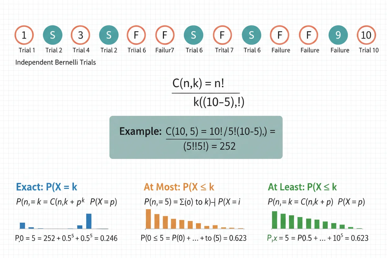
Binomial probability measures the chance of obtaining a specified number of successes in a fixed number of repeated trials when each trial has two possible outcomes, the trials are independent, and the probability of success remains constant. It is commonly used for questions such as the probability that exactly 4 of 10 customers respond, at most 2 components are defective, or at least 1 person in a group has a particular characteristic. The central binomial probability formula combines the probability of one success-failure arrangement with the number of different arrangements that produce the same number of successes. Exact probabilities use the binomial probability mass function directly, while “at most,” “at least,” and range questions require adding several exact probabilities or using complements. Correct calculations depend on translating phrases such as “more than,” “no more than,” and “at least” into the appropriate mathematical event. The method should only be applied when its fixed-trial, binary-outcome, independence, and constant-probability assumptions reasonably describe the process.
Binomial probability is the calculation-focused counterpart to the broader binomial distribution, which describes the distribution’s PMF, CDF, support, parameters, mean, variance, and overall shape. Both belong within core statistics and the wider Statistics & Probability framework.
What Is Binomial Probability?
Binomial probability is the probability that a binomial random variable takes a particular value or falls within a specified set of values.
If X represents the number of successes in n trials, then:
X ~ Bin(n, p)
where:
- n = number of trials
- p = probability of success on each trial
- 1 − p = probability of failure
- X = number of successes
The possible values are:
X = 0, 1, 2, …, n
An exact binomial probability has the form:
P(X = x)
A cumulative or range calculation may instead ask for:
P(X ≤ x)
P(X ≥ x)
P(a ≤ X ≤ b)
The wording of the problem determines which event must be calculated.
Binomial Probability Formula
The probability of obtaining exactly x successes in n independent trials is:
P(X = x) = C(n, x)pˣ(1 − p)ⁿ⁻ˣ
where:
C(n, x) = n!/[x!(n − x)!]
The combination term C(n, x), sometimes written “n choose x,” counts the number of distinct ways x successes can be positioned among n trials.
The rest of the formula gives the probability of each arrangement:
pˣ = probability contribution from x successes
(1 − p)ⁿ⁻ˣ = probability contribution from n − x failures
Therefore, binomial probability is built from:
Number of valid arrangements × Probability of each arrangement
Conditions for Using Binomial Probability
Before applying the formula, verify that the process actually satisfies the binomial model.
The Number of Trials Is Fixed
There must be a predetermined number n of trials.
For example, asking about the number of defective products among 20 inspected products has:
n = 20
A process that continues until a success occurs does not have a fixed number of trials and is not an ordinary binomial experiment.
Each Trial Has Two Relevant Outcomes
Each trial must be classified into two mutually exclusive outcomes, conventionally called success and failure.
Examples include:
- pass or fail
- defective or nondefective
- response or no response
- yes or no
- success or failure
“Success” is simply the event being counted. It does not imply that the outcome is desirable.
Trials Are Independent
The outcome of one trial must not alter the probability of success on another trial.
If one observation changes subsequent probabilities, the independence assumption is violated.
Sampling without replacement can be an important example. If objects are drawn from a small finite population without replacement, the probability changes from one draw to the next, so an exact binomial model may not be appropriate.
The Success Probability Is Constant
Every trial must have the same probability p of success.
If:
p = 0.30
on the first trial, the ordinary binomial model assumes the same value on every other trial.
When trial probabilities differ substantially, the standard binomial probability formula does not apply exactly.
Why the Combination Formula Is Necessary
Suppose five trials contain exactly two successes.
One sequence could be:
S S F F F
Another could be:
S F S F F
Another could be:
F F S S F
Every sequence with exactly two successes has probability:
p²(1 − p)³
assuming independent trials with constant p.
However, there is more than one arrangement containing exactly two successes.
The number of arrangements is:
C(5, 2) = 5!/[2!3!]
C(5, 2) = 10
Therefore:
P(X = 2) = 10p²(1 − p)³
Without C(n, x), the calculation would give the probability of only one particular ordering rather than the probability of obtaining x successes in any order.
Example 1: Probability of Exactly x Successes
Suppose eight independent customers each have a 30% probability of purchasing a product.
Let:
X = number of customers who purchase
Then:
X ~ Bin(8, 0.30)
What is the binomial probability that exactly three customers purchase?
We want:
P(X = 3)
Apply the formula:
P(X = 3) = C(8, 3)(0.30)³(0.70)⁵
Calculate the combination:
C(8, 3) = 8!/[3!5!]
C(8, 3) = 56
Now calculate the probability:
P(X = 3) = 56(0.30)³(0.70)⁵
P(X = 3) ≈ 0.2541
Therefore:
P(X = 3) ≈ 25.41%
The probability that exactly three of the eight customers purchase is approximately 25.41%.
Notice that this is an exact probability. It does not include two customers, four customers, or any other number of successes.
How to Translate Binomial Probability Wording
Many errors occur before the arithmetic begins because verbal phrases are translated incorrectly.
| Phrase | Mathematical event |
|---|---|
| Exactly x | X = x |
| At most x | X ≤ x |
| No more than x | X ≤ x |
| At least x | X ≥ x |
| No fewer than x | X ≥ x |
| More than x | X > x |
| Fewer than x | X < x |
| Between a and b inclusive | a ≤ X ≤ b |
| At least one | X ≥ 1 |
| None | X = 0 |
Because X is an integer-valued count:
X < 4
is equivalent to:
X ≤ 3
and:
X > 4
is equivalent to:
X ≥ 5
This discrete structure makes endpoint wording especially important.
Example 2: Binomial Probability of At Most x
Continue with:
X ~ Bin(8, 0.30)
Suppose we want the probability of at most two successes.
“At most two” means:
X ≤ 2
Therefore:
P(X ≤ 2) = P(X = 0) + P(X = 1) + P(X = 2)
Using the binomial formula:
P(X = 0) = C(8, 0)(0.30)⁰(0.70)⁸
P(X = 1) = C(8, 1)(0.30)¹(0.70)⁷
P(X = 2) = C(8, 2)(0.30)²(0.70)⁶
Adding the values gives:
P(X ≤ 2) ≈ 0.5518
Therefore:
P(X ≤ 2) ≈ 55.18%
This is a cumulative binomial probability because several possible success counts are included.
The binomial distribution describes this cumulative structure through its CDF; here, the important calculation rule is that “at most x” includes every integer from 0 through x.
Example 3: Binomial Probability of At Least x
Using the same model:
X ~ Bin(8, 0.30)
suppose we want the probability of at least three successes.
This means:
P(X ≥ 3)
One method is to add:
P(X = 3) + P(X = 4) + … + P(X = 8)
However, the complement is shorter:
P(X ≥ 3) = 1 − P(X ≤ 2)
From the previous example:
P(X ≤ 2) ≈ 0.5518
Therefore:
P(X ≥ 3) = 1 − 0.5518
P(X ≥ 3) ≈ 0.4482
So the probability of three or more successes is approximately:
44.82%
Using a complement often reduces the number of calculations substantially.
The Complement Rule
The complement rule is one of the most useful tools in binomial probability.
For any event A:
P(Aᶜ) = 1 − P(A)
For a binomial random variable:
P(X ≥ x) = 1 − P(X ≤ x − 1)
Similarly:
P(X > x) = 1 − P(X ≤ x)
and:
P(X < x) = P(X ≤ x − 1)
The distinction between x and x − 1 matters because the binomial random variable is discrete.
For example:
P(X ≥ 3) = 1 − P(X ≤ 2)
not:
P(X ≥ 3) = 1 − P(X ≤ 3)
The latter incorrectly removes the probability of exactly three successes.
Example 4: Probability of At Least One Success
“At least one” is a particularly useful case for the complement rule.
Suppose six independent attempts each have success probability:
p = 0.20
Let:
X ~ Bin(6, 0.20)
We want:
P(X ≥ 1)
The complement of at least one success is zero successes:
P(X ≥ 1) = 1 − P(X = 0)
Now:
P(X = 0) = C(6, 0)(0.20)⁰(0.80)⁶
Because:
C(6, 0) = 1
and:
(0.20)⁰ = 1
we obtain:
P(X = 0) = (0.80)⁶
P(X = 0) = 0.262144
Therefore:
P(X ≥ 1) = 1 − 0.262144
P(X ≥ 1) = 0.737856
So the probability of at least one success is approximately:
73.79%
Calculating six separate probabilities for one through six successes would produce the same answer, but the complement is much more efficient.
Example 5: Probability Between Two Values
Suppose:
X ~ Bin(10, 0.40)
What is the probability of obtaining between two and five successes, inclusive?
The event is:
2 ≤ X ≤ 5
Therefore:
P(2 ≤ X ≤ 5) = P(X = 2) + P(X = 3) + P(X = 4) + P(X = 5)
Evaluating these terms gives:
P(2 ≤ X ≤ 5) ≈ 0.7874
Therefore:
P(2 ≤ X ≤ 5) ≈ 78.74%
Using cumulative probabilities, the same event can be written:
P(2 ≤ X ≤ 5) = P(X ≤ 5) − P(X ≤ 1)
Both methods are mathematically equivalent.
Exact vs Cumulative Binomial Probability
An exact binomial probability refers to one count:
P(X = x)
A cumulative binomial probability combines several counts:
P(X ≤ x)
or another range of values.
For example:
P(X = 4)
means exactly four successes.
By contrast:
P(X ≤ 4)
includes:
X = 0, 1, 2, 3, 4
Confusing these two forms can produce a numerically plausible but conceptually incorrect result.
Before substituting values into the formula, identify the event explicitly.
How to Calculate Binomial Probability Step by Step
A reliable calculation process is:
Step 1: Identify n
Determine the fixed number of trials.
Step 2: Identify p
Determine the probability of success on each trial.
Step 3: Define X
State exactly what the random variable counts.
For example:
X = number of defective products among 12 inspected products
Step 4: Translate the Wording
Convert the verbal question into probability notation.
For example:
“At least four” becomes:
P(X ≥ 4)
Step 5: Decide Whether to Use Direct Addition or a Complement
A short sum may be easiest directly.
A long upper-tail calculation is often easier with:
1 − P(complement)
Step 6: Use the Binomial Formula for Each Required Exact Value
P(X = x) = C(n, x)pˣ(1 − p)ⁿ⁻ˣ
Step 7: Add or Subtract as Required
Combine exact probabilities according to the event.
Step 8: Round Only at the End
Retaining more digits during intermediate calculations reduces avoidable rounding error.
Binomial Probability With Percentages
Probabilities given as percentages must first be converted to decimals.
For example:
35% = 0.35
Therefore, if n = 12 and p = 35%:
X ~ Bin(12, 0.35)
Using p = 35 directly would be incorrect because probability values must lie between 0 and 1.
Likewise:
7% = 0.07
2.5% = 0.025
80% = 0.80
The final answer can then be converted back to a percentage if that makes interpretation clearer.
Binomial Probability for Zero Successes
The zero-success case simplifies considerably.
Starting from:
P(X = x) = C(n, x)pˣ(1 − p)ⁿ⁻ˣ
set:
x = 0
Then:
P(X = 0) = C(n, 0)p⁰(1 − p)ⁿ
Because:
C(n, 0) = 1
and:
p⁰ = 1
we obtain:
P(X = 0) = (1 − p)ⁿ
This formula is especially useful when calculating the probability of at least one success:
P(X ≥ 1) = 1 − (1 − p)ⁿ
Binomial Probability for All Successes
At the opposite extreme:
X = n
so:
P(X = n) = C(n, n)pⁿ(1 − p)⁰
Since:
C(n, n) = 1
and:
(1 − p)⁰ = 1
we obtain:
P(X = n) = pⁿ
For example, if five independent trials each have success probability 0.8:
P(X = 5) = (0.8)⁵
P(X = 5) = 0.32768
Thus, even a fairly high per-trial success probability does not guarantee that every trial succeeds.
Binomial Probability and Expected Value
The probability calculation for a particular event should not be confused with the expected number of successes.
For:
X ~ Bin(n, p)
the mean is:
E(X) = np
Suppose:
n = 20
and:
p = 0.40
Then:
E(X) = 20 × 0.40 = 8
This means the long-run average success count is eight across repeated sets of 20 trials.
It does not mean:
P(X = 8) = 1
Nor does it imply that eight successes must be the observed result in any particular experiment.
Expected value describes the center of the distribution; binomial probability quantifies the chance of specified outcomes.
Binomial Probability and Independence
Independence is not simply a technical detail. It is what allows trial probabilities to multiply in the form used by the binomial formula.
For a particular sequence containing x successes and n − x failures:
P(sequence) = pˣ(1 − p)ⁿ⁻ˣ
This multiplication relies on the relevant independence assumptions.
If earlier outcomes alter later probabilities, the probability of a sequence generally cannot be represented with a single constant p in this way.
For example, repeated draws from a deck without replacement are dependent because removing one card changes the composition of the deck.
Sampling Without Replacement
Suppose a finite population contains some successful and unsuccessful items, and a sample is drawn without replacement.
Strictly speaking, those draws are dependent. After each item is removed, the success probability for the next draw can change.
When the sampled fraction is extremely small relative to the population, treating the trials as approximately independent may sometimes produce a close approximation.
However, that is an approximation rather than an exact binomial model.
The decision should be based on the sampling structure and required precision rather than automatically applying the familiar formula.
Binomial Probability vs Binomial Distribution
The terms are related but describe different levels of the problem.
The binomial distribution is the complete probability distribution of:
X ~ Bin(n, p)
It includes the support, PMF, CDF, mean, variance, shape, and other properties.
Binomial probability usually refers to calculating the probability of a specific event under that distribution, such as:
P(X = 5)
P(X ≤ 5)
P(X ≥ 5)
The binomial distribution therefore provides the underlying model, while binomial probability focuses on using that model to answer specific probability questions.
Binomial Probability and Bayes’ Theorem
Bayes’ theorem and binomial probability can appear in the same analysis but perform different functions.
Binomial probability may provide the likelihood of observed count data under a proposed success probability.
For example:
P(X = 7|p = 0.6)
can be calculated with the binomial formula.
Bayes’ theorem can then combine that likelihood with prior information to update probabilities assigned to competing hypotheses or parameter values.
Thus, binomial probability can supply evidence used inside a Bayesian calculation, but the two formulas answer different conditional-probability questions.
Binomial Probability and Confidence Intervals
Suppose x successes are observed in n trials.
The observed sample proportion is:
p̂ = x/n
This provides a point estimate of an unknown population success probability p.
A confidence interval addresses a different question: how much sampling uncertainty surrounds that estimate under a specified procedure?
Binomial probability assumes a particular p when calculating probabilities such as P(X = x). Confidence-interval estimation treats p as an unknown parameter to be estimated from observed data.
Keeping those roles separate avoids confusing probability calculations with parameter estimation.
Binomial Probability vs Chi-Square
A chi-square test typically analyzes categorical counts through a chi-square reference distribution, often for goodness-of-fit or association questions.
Binomial probability is more narrowly designed around the number of successes in repeated binary trials.
If the outcome has only success and failure categories and a specific success probability is assumed, an exact binomial calculation may directly model the count.
When several categories or contingency-table relationships are involved, a chi-square procedure may address the appropriate inferential question instead.
The correct method depends on the structure of the data and the hypothesis being tested.
Binomial Probability vs ANOVA
ANOVA typically compares means of quantitative outcomes across groups.
Binomial probability models counts of successes under repeated binary trials.
For example, suppose three teaching methods produce numerical examination scores. Comparing their population mean scores may call for ANOVA.
If instead the outcome is whether each student passes or fails and the question concerns a count of passes under a specified success probability, a binomial model may be relevant.
These methods are not substitutes. They address different response types and different statistical questions.
Statistical Inference From Binomial Data
A binomial probability can also be used to assess how unusual an observed success count would be under a stated model.
Suppose a null model specifies:
p = 0.50
and an experiment produces an unusually large number of successes.
Exact probabilities under:
X ~ Bin(n, 0.50)
can help quantify how extreme that observation is relative to the null model.
However, inferential interpretation requires more than reporting P(X = x). A hypothesis test typically considers outcomes at least as inconsistent with H₀ as the observed result according to a specified test statistic and alternative hypothesis.
An exact observed probability is therefore not automatically a p-value.
This distinction is important in discrete hypothesis testing.
Probability Is Not Evidence of Causation
A binomial probability calculation describes the probability of outcomes under a specified model.
It does not establish why a success probability has a particular value.
For example, finding that a success count would be unusual under p = 0.20 may provide evidence that the stated probability model is questionable. It does not by itself identify the mechanism responsible for the discrepancy.
Association, probability, model fit, and causation are separate concepts.
Common Binomial Probability Mistakes
One common mistake is applying the formula when the trials are not independent or the success probability changes.
Another is forgetting the combination term:
C(n, x)
Without it, the calculation generally represents only one particular arrangement of successes and failures.
A third mistake is using:
pⁿ
for exactly x successes when x is not n. The correct formula must include both successes and failures.
Another frequent error is confusing:
P(X ≥ x)
with:
1 − P(X ≤ x)
The correct relationship is:
P(X ≥ x) = 1 − P(X ≤ x − 1)
Similarly:
P(X > x) = 1 − P(X ≤ x)
These formulas differ by one entire probability mass.
Rounding intermediate probabilities too aggressively can also create noticeable error when many terms are added.
Finally, a small binomial probability should not automatically be interpreted as proof that an assumed model is false. Statistical inference requires a defined hypothesis-testing framework and consideration of which outcomes count as equally or more extreme.
Choosing Direct Addition or a Complement
The most efficient method depends on the number of terms required.
If the event is:
P(X ≤ 2)
adding:
P(X = 0) + P(X = 1) + P(X = 2)
is straightforward.
If the event is:
P(X ≥ 2)
and n is large, adding every probability from 2 through n would be inefficient.
Instead:
P(X ≥ 2) = 1 − P(X ≤ 1)
The complement reduces the calculation to only two exact probabilities.
A useful principle is to calculate whichever side of the distribution contains fewer terms, then use the complement if necessary.
How to Interpret the Final Binomial Probability
A binomial probability should be interpreted in the context of repeated experiments under the stated assumptions.
Suppose:
P(X = 3) ≈ 0.2541
This means that under the specified n and p, repeated independent experiments of the same structure would produce exactly three successes about 25.41% of the time in the long run.
It does not mean that 25.41% of the individual trials are successes.
That per-trial probability is p.
The binomial result applies to the success count across the entire set of trials.
Frequently Asked Questions About Binomial Probability
What is binomial probability?
Binomial probability is the probability of obtaining a specified number or range of successes in a fixed number of independent binary trials with constant success probability p.
What is the binomial probability formula?
For exactly x successes:
P(X = x) = C(n, x)pˣ(1 − p)ⁿ⁻ˣ
where:
C(n, x) = n!/[x!(n − x)!]
What does n mean in binomial probability?
n is the fixed total number of trials.
What does x mean?
x is the number of successes whose probability is being calculated.
For an exact probability:
x ∈ {0, 1, 2, …, n}
What does p mean?
p is the probability of success on each trial. A standard binomial model assumes that the same p applies to every trial.
How do you calculate exactly x successes?
Use:
P(X = x) = C(n, x)pˣ(1 − p)ⁿ⁻ˣ
Only the single value x is included.
How do you calculate at most x successes?
“At most x” means:
P(X ≤ x)
Add the probabilities from zero through x:
P(X ≤ x) = Σₖ₌₀ˣ P(X = k)
How do you calculate at least x successes?
“At least x” means:
P(X ≥ x)
A convenient complement is:
P(X ≥ x) = 1 − P(X ≤ x − 1)
How do you calculate at least one success?
Use:
P(X ≥ 1) = 1 − P(X = 0)
which simplifies to:
P(X ≥ 1) = 1 − (1 − p)ⁿ
What is the difference between “at least” and “more than”?
“At least x” includes x:
X ≥ x
“More than x” excludes x:
X > x
For integer-valued X:
X > x
is equivalent to:
X ≥ x + 1
What is the difference between “at most” and “less than”?
“At most x” means:
X ≤ x
“Less than x” means:
X < x
For an integer-valued binomial variable:
X < x
is equivalent to:
X ≤ x − 1
Why is C(n, x) included in the formula?
C(n, x) counts how many different trial sequences contain exactly x successes. The probability of each sequence is multiplied by this number to obtain the probability of x successes in any order.
Can binomial probability be used when trials are dependent?
Not exactly under the standard model. Independence is one of the defining binomial assumptions. Dependent observations may require another probability model.
Can the success probability change between trials?
Not in an ordinary binomial model. The same success probability p must apply to each trial.
Is an exact binomial probability the same as a p-value?
No. P(X = x) gives the probability of one exact count under the model. A p-value generally includes the observed result and outcomes considered at least as extreme under a specified null hypothesis and test procedure.
What is the difference between binomial probability and the binomial distribution?
Binomial probability focuses on calculating specific events such as exactly x, at most x, or at least x successes. The binomial distribution describes the complete random-variable model, including its PMF, CDF, parameters, support, mean, variance, and shape.




