


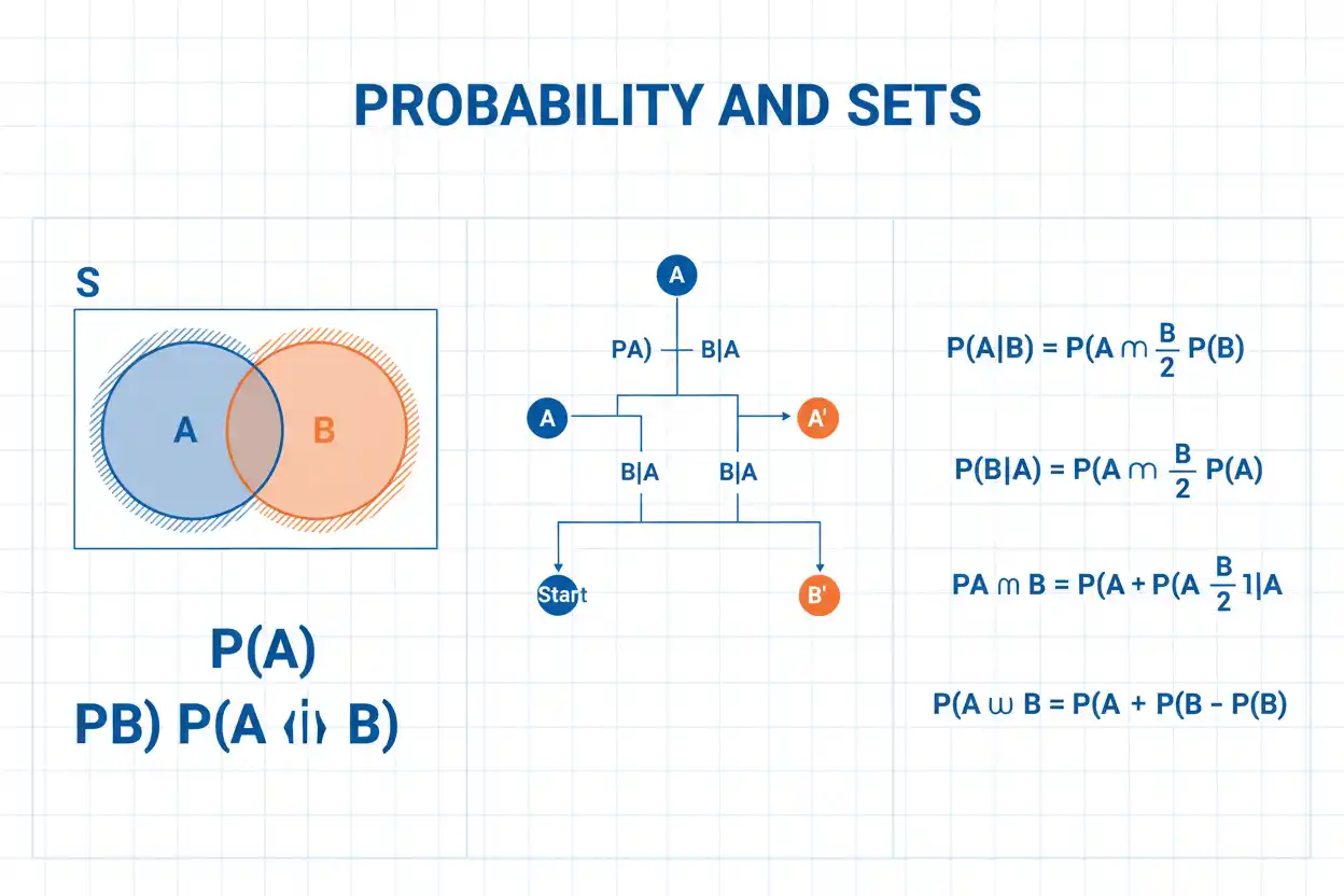
Probability is the mathematical framework used to quantify uncertainty by assigning numerical values to possible events, with values ranging from 0 for an impossible event to 1 for a certain event. A probability can describe the chance of a single event, the likelihood that several events occur together, the chance that at least one of several events occurs, or how an event’s likelihood changes after new information becomes available. The basic rules of probability apply across many areas of statistics, from simple coin and card examples to sampling, regression, hypothesis testing, reliability, forecasting, and probability distributions such as the Poisson distribution. Although many introductory problems can be solved by counting equally likely outcomes, probability is broader than simple counting because events may have unequal likelihoods and may depend on one another. Understanding complements, unions, intersections, conditional probability, independence, and the multiplication and addition rules is therefore essential before moving to more specialized statistical models. Correct probability calculations also require clearly defining the sample space and events, because a formula can be applied perfectly while still answering the wrong question if the event itself has been specified incorrectly.
Probability is one of the central foundations of core statistics and the wider Statistics & Probability framework. It provides the mathematical language underlying discrete models such as the Poisson distribution, while ordered summaries such as quartiles and percentiles describe positions within data or probability distributions rather than the rules that determine event likelihood itself.
What Is Probability?
Probability measures how likely an event is to occur.
For an event A:
0 ≤ P(A) ≤ 1
where:
- P(A) = probability of event A
- 0 = impossible
- 1 = certain
A probability of:
0.25
can also be written as:
25%
while:
0.80
corresponds to:
80%
The closer probability is to 1, the more likely the event. The closer it is to 0, the less likely the event.
A value between 0 and 1 does not guarantee what will happen in one individual trial. It describes uncertainty across possible outcomes or repeated comparable situations.
Basic Probability Formula
When all outcomes in a finite sample space are equally likely, the basic probability formula is:
P(A) = Number of favorable outcomes / Total number of possible outcomes
Suppose a fair six-sided die is rolled.
The sample space is:
S = {1, 2, 3, 4, 5, 6}
If event A is:
rolling an even number
then:
A = {2, 4, 6}
There are:
3 favorable outcomes
out of:
6 total outcomes.
Therefore:
P(A) = 3/6
P(A) = 1/2
P(A) = 0.50
Thus, the probability of rolling an even number is:
50%
Sample Space
The sample space contains all possible outcomes of the experiment.
It is commonly represented by:
S
For one fair coin toss:
S = {H, T}
For one six-sided die:
S = {1,2,3,4,5,6}
For two coin tosses:
S = {HH, HT, TH, TT}
A probability problem cannot be interpreted correctly unless the relevant sample space is understood.
For two coins, for example, saying:
“one head and one tail”
corresponds to two distinct equally likely outcomes:
HT
and:
TH
rather than one.
Events
An event is a subset of the sample space.
Suppose:
S = {1,2,3,4,5,6}
for a die roll.
Event A might be:
A = {2,4,6}
representing an even number.
Event B might be:
B = {4,5,6}
representing a result greater than 3.
Events can:
- overlap,
- be mutually exclusive,
- contain one another,
- include the whole sample space,
- contain no outcomes.
Probability rules describe how these event sets interact.
Impossible and Certain Events
The empty event:
∅
contains no outcomes, so:
P(∅) = 0
The complete sample space S contains every possible outcome, so:
P(S) = 1
These are fundamental probability axioms.
An event with probability zero is impossible in a finite discrete model, although continuous probability requires more care because an individual point can have probability zero without being logically impossible.
Similarly, an event with probability one is almost sure under a general probability model, although exceptional measure-zero outcomes can still require technical distinction in advanced theory.
Complement Rule
The complement of event A, written:
Aᶜ
contains all outcomes in the sample space that are not in A.
The complement rule is:
P(Aᶜ) = 1 − P(A)
Equivalently:
P(A) + P(Aᶜ) = 1
If:
P(A) = 0.70
then:
P(Aᶜ) = 1 − 0.70
P(Aᶜ) = 0.30
The complement rule is especially useful for events such as:
at least one
because it is often easier to calculate the probability of none and subtract from 1.
Complement Example
Suppose a component has probability:
0.08
of failing during a specified period.
Then the probability that it does not fail is:
1 − 0.08
= 0.92
Therefore:
P(no failure) = 92%
The two events are complements because exactly one must occur under the specified model.
Addition Rule
The probability that A or B occurs is written:
P(A ∪ B)
The general addition rule is:
P(A ∪ B) = P(A) + P(B) − P(A ∩ B)
The intersection:
A ∩ B
represents outcomes belonging to both A and B.
The overlap must be subtracted because adding P(A) and P(B) counts those shared outcomes twice.
Addition Rule Example
Roll one fair die.
Let:
A = even result = {2,4,6}
and:
B = result greater than 3 = {4,5,6}
Then:
P(A) = 3/6
P(B) = 3/6
Their intersection is:
A ∩ B = {4,6}
so:
P(A ∩ B) = 2/6
Therefore:
P(A ∪ B) = 3/6 + 3/6 − 2/6
= 4/6
= 2/3
The event A or B is:
{2,4,5,6}
which confirms the result.
Mutually Exclusive Events
Two events are mutually exclusive when they cannot occur simultaneously.
Therefore:
A ∩ B = ∅
and:
P(A ∩ B) = 0
For mutually exclusive events, the addition rule simplifies to:
P(A ∪ B) = P(A) + P(B)
On one die roll, the events:
A = roll a 2
and:
B = roll a 5
are mutually exclusive.
Therefore:
P(A or B) = 1/6 + 1/6
= 2/6
= 1/3
Mutually Exclusive Does Not Mean Independent
Mutual exclusivity and independence are different concepts.
If two events with positive probability are mutually exclusive, then observing one tells us the other did not occur.
Therefore, they cannot be independent.
Suppose:
P(A) > 0
P(B) > 0
and:
A ∩ B = ∅
Then:
P(A ∩ B) = 0
But if A and B were independent, we would need:
P(A ∩ B) = P(A)P(B)
which would be positive.
Therefore, nontrivial mutually exclusive events are dependent.
This distinction is one of the most common sources of probability errors.
Intersection
The intersection:
A ∩ B
means:
A and B both occur.
For example, suppose a randomly selected card is drawn from a standard 52-card deck.
Let:
A = card is a heart
and:
B = card is a face card.
The cards satisfying both events are:
Jack of hearts
Queen of hearts
King of hearts
Therefore:
P(A ∩ B) = 3/52
Intersections are central to both multiplication rules and conditional probability.
Conditional Probability
Conditional probability measures the probability of A after learning that B occurred.
It is written:
P(A|B)
and calculated as:
P(A|B) = P(A ∩ B)/P(B)
provided:
P(B) > 0
Conditioning changes the reference sample space.
Instead of considering every possible outcome, we restrict attention to outcomes inside B and ask what proportion of those also belong to A.
Conditional Probability Example
Draw one card from a standard 52-card deck.
Let:
A = card is a king
and:
B = card is a face card.
There are:
12 face cards
in total:
4 jacks, 4 queens, 4 kings.
Among those 12 face cards:
4
are kings.
Therefore:
P(A|B) = 4/12
= 1/3
Using the formula:
P(A ∩ B) = 4/52
and:
P(B) = 12/52
so:
P(A|B) = (4/52)/(12/52)
= 4/12
= 1/3
Learning that the selected card is a face card increases the probability that it is a king from:
4/52 = 1/13
to:
1/3.
Multiplication Rule
Rearranging the conditional probability formula gives:
P(A ∩ B) = P(A|B)P(B)
Equivalently:
P(A ∩ B) = P(B|A)P(A)
This is the general multiplication rule.
It applies whether or not the events are independent.
The conditional term accounts for any dependence between the events.
Multiplication Rule Example
Suppose a container has:
5 red objects
and:
3 blue objects.
Two objects are selected without replacement.
What is the probability both are red?
Probability first is red:
5/8
After one red object is removed, there are:
4 red
among:
7 total.
Therefore:
P(second red | first red) = 4/7
Multiply:
P(both red) = (5/8)(4/7)
= 20/56
= 5/14
≈ 0.3571
The draws are dependent because the first selection changes the composition of the container.
Independent Events
Events A and B are independent when knowing one occurred does not change the probability of the other.
Mathematically:
P(A|B) = P(A)
when P(B) > 0.
An equivalent condition is:
P(A ∩ B) = P(A)P(B)
Suppose two fair coins are tossed.
Let:
A = first coin is heads
and:
B = second coin is heads.
Then:
P(A) = 1/2
P(B) = 1/2
and:
P(A ∩ B) = 1/4
Since:
(1/2)(1/2) = 1/4
the events are independent.
Independence Example With Repeated Trials
Suppose a fair die is rolled twice.
The probability of rolling a 6 on the first roll is:
1/6
The probability of rolling a 6 on the second roll is also:
1/6
Assuming independent rolls:
P(two sixes) = (1/6)(1/6)
= 1/36
The first roll does not change the distribution of the second.
This differs from sampling without replacement, where the available outcomes change after each draw.
At Least One Event
Problems involving:
at least one
are often easiest with complements.
Suppose an event has probability:
p
on each independent trial.
The probability it does not occur on one trial is:
1 − p
The probability it never occurs in n independent trials is:
(1 − p)^n
Therefore:
P(at least one occurrence) = 1 − (1 − p)^n
This formula is one of the most useful applications of the complement rule.
At Least One Example
Suppose the probability of an event on each independent trial is:
p = 0.20
There are:
n = 4
trials.
Probability of no occurrences:
(1 − 0.20)^4
= 0.8^4
= 0.4096
Therefore:
P(at least one) = 1 − 0.4096
= 0.5904
Thus:
P(at least one) = 59.04%
Adding separate probabilities for one, two, three, and four occurrences would produce the same result but would require considerably more work.
Exactly One Occurrence
For n independent Bernoulli trials with event probability p, the probability of exactly one occurrence is:
P(X=1) = C(n,1)p(1−p)^(n−1)
Since:
C(n,1) = n
we can write:
P(X=1) = np(1−p)^(n−1)
For:
n = 4
and:
p = 0.20
we obtain:
P(X=1) = 4(0.20)(0.80³)
= 0.4096
Notice that this is different from the probability of at least one occurrence:
0.5904
because the latter also includes two, three, or four occurrences.
Probability Trees
A probability tree represents sequential events using branches.
Suppose an event A can occur with:
P(A)
and not occur with:
P(Aᶜ).
After each branch, a second event B can have conditional probabilities such as:
P(B|A)
and:
P(B|Aᶜ).
The probability of a complete path is found by multiplying branch probabilities.
For example:
P(A ∩ B) = P(A)P(B|A)
Probabilities from mutually exclusive terminal paths can then be added.
Probability trees are especially useful for sequential conditional problems where the sample structure changes over stages.
Law of Total Probability
Suppose events:
B₁, B₂, …, Bₖ
form a partition of the sample space, meaning they are mutually exclusive and collectively exhaustive.
Then:
P(A) = ΣP(A|Bᵢ)P(Bᵢ)
This is the law of total probability.
It expresses the overall probability of A as a weighted combination of conditional probabilities across mutually exclusive cases.
The weights are the probabilities of the cases themselves.
Total Probability Example
Suppose:
60%
of items come from Machine 1 and:
40%
from Machine 2.
Let:
P(defect | Machine 1) = 0.02
and:
P(defect | Machine 2) = 0.05
Then:
P(defect) = 0.02(0.60) + 0.05(0.40)
= 0.012 + 0.020
= 0.032
Therefore:
P(defect) = 3.2%
The overall defect probability is a weighted average of the machine-specific conditional probabilities.
Bayes’ Rule
Conditional probability can be reversed through Bayes’ theorem:
P(A|B) = P(B|A)P(A)/P(B)
where:
P(B) > 0
If B can arise through several mutually exclusive cases, the denominator can be calculated using the law of total probability.
Bayes’ theorem is especially useful when the probability of evidence given a cause is known but the desired quantity is the probability of the cause given the evidence.
The conditional direction matters. In general:
P(A|B) ≠ P(B|A)
Bayes Example
Suppose:
P(D) = 0.02
for a condition D.
A test has:
P(positive | D) = 0.90
and:
P(positive | Dᶜ) = 0.05
The total probability of a positive result is:
P(positive) = 0.90(0.02) + 0.05(0.98)
= 0.018 + 0.049
= 0.067
Therefore:
P(D | positive) = 0.018/0.067
≈ 0.2687
So the conditional probability is approximately:
26.87%
despite the test’s 90% sensitivity.
The relatively low prior probability and false-positive rate both matter.
Joint Probability
Joint probability refers to the probability of events occurring together.
For two events:
P(A ∩ B)
For three events:
P(A ∩ B ∩ C)
Sequentially:
P(A ∩ B ∩ C) = P(A)P(B|A)P(C|A∩B)
If A, B, and C are mutually independent, this simplifies to:
P(A ∩ B ∩ C) = P(A)P(B)P(C)
Independence is what allows the conditional terms to be replaced by unconditional probabilities.
Pairwise vs Mutual Independence
Three events can be pairwise independent without being mutually independent.
Pairwise independence requires:
P(A∩B) = P(A)P(B)
P(A∩C) = P(A)P(C)
P(B∩C) = P(B)P(C)
Mutual independence additionally requires the corresponding relationship for every combination, including:
P(A∩B∩C) = P(A)P(B)P(C)
This distinction becomes important in more advanced probability models.
Checking only pairs does not always establish full independence.
Counting Outcomes
When outcomes are equally likely, combinatorial counting can simplify probability calculations.
The number of ways to choose r objects from n without regard to order is:
C(n,r) = n!/[r!(n−r)!]
For example:
C(5,2) = 5!/[2!3!]
= 10
This tells us there are ten distinct ways to choose two objects from five.
Counting formulas are especially useful in binomial, hypergeometric, and card-selection problems.
Permutations
When order matters, the number of ordered arrangements of r objects selected from n is:
P(n,r) = n!/(n−r)!
For example, choosing first, second, and third places from ten participants gives:
P(10,3) = 10!/7!
= 10×9×8
= 720
Combinations and permutations solve different counting questions.
Using the wrong one changes the sample-space size and therefore the resulting probability.
Equally Likely Outcomes Are an Assumption
The basic formula:
favorable outcomes / total outcomes
works only when the outcomes being counted are equally likely.
Suppose a loaded die has:
P(6) = 0.40
while the remaining probabilities are distributed across outcomes 1 through 5.
Then counting:
one favorable face / six faces
would incorrectly give:
1/6
for rolling a 6.
Probability must use the actual distribution:
P(6) = 0.40
Counting alone cannot handle unequal outcome probabilities unless those weights are explicitly incorporated.
Empirical Probability
Probability can be estimated from observed relative frequency.
If an event occurs x times in n observations:
p̂ = x/n
Suppose an event occurs:
37 times
in:
100 trials.
The empirical probability estimate is:
p̂ = 37/100
= 0.37
This does not mean the true population probability is known to be exactly 0.37.
It is a sample estimate subject to random variation and any limitations in how the observations were collected.
Theoretical vs Empirical Probability
Theoretical probability comes from a specified mathematical model.
For a fair coin:
P(heads) = 0.50
Empirical probability comes from observed frequency.
If 1,000 coin tosses produce:
487 heads
then:
p̂ = 487/1000
= 0.487
The empirical value need not equal 0.50 exactly.
Sampling variation creates differences between observed relative frequencies and theoretical probabilities.
As the number of suitable independent trials grows, empirical frequency often becomes increasingly stable around the underlying probability under appropriate conditions.
Law of Large Numbers
The law of large numbers explains why repeated averages or relative frequencies tend to stabilize around theoretical expectations under suitable assumptions.
For independent Bernoulli trials with event probability p:
Xᵢ ∈ {0,1}
and:
E(Xᵢ) = p
The sample proportion:
p̂ = (X₁ + … + Xₙ)/n
converges toward:
p
as n becomes large under standard conditions.
This does not mean short sequences must look balanced.
A fair coin can produce several heads in a row without violating its 50% probability.
Gambler’s Fallacy
The gambler’s fallacy is the mistaken belief that independent events must immediately compensate for recent outcomes.
Suppose a fair coin produces:
H, H, H, H, H
The probability of heads on the next independent toss remains:
0.50
It does not become smaller merely because heads occurred several times previously.
The long-run law of large numbers does not create a short-run corrective force.
Independence means the next outcome retains its original probability.
Conditional Dependence
Events can be dependent because knowledge of one changes the probability of another.
Suppose:
P(A) = 0.40
but:
P(A|B) = 0.70
Then observing B materially changes the probability of A.
Therefore A and B are dependent.
Dependence can arise through causal relationships, common causes, sampling without replacement, time structure, spatial clustering, or shared environmental factors.
Ignoring dependence can make multiplication formulas and uncertainty calculations incorrect.
Probability Distributions
A probability distribution assigns probabilities across the possible values of a random variable.
For a discrete random variable:
P(X=x)
is a probability mass function.
For a continuous random variable:
f(x)
is a density function, and interval probabilities are areas under that density.
For example, the Poisson distribution assigns probability to count values:
0,1,2,3,…
using:
P(X=k) = e^−λ λ^k/k!
The general rules of probability remain valid regardless of which distribution supplies the event probabilities.
Random Variables
A random variable assigns numerical values to outcomes of a random experiment.
A discrete random variable takes countable values.
Examples include:
number of arrivals
number of successes
number of defects
A continuous random variable can take values over an interval.
Examples include:
time
height
temperature
Probability distributions describe how probability is allocated over these possible numerical values.
Expected Value
For a discrete random variable X:
E(X) = ΣxP(X=x)
provided the sum exists.
Expected value is a probability-weighted mean.
Suppose X takes:
0 with probability 0.25
1 with probability 0.50
2 with probability 0.25
Then:
E(X) = 0(0.25) + 1(0.50) + 2(0.25)
= 1
The expected value need not be an outcome that occurs in every trial. It represents a long-run probability-weighted average.
Variance of a Random Variable
If:
μ = E(X)
then:
Var(X) = E[(X−μ)²]
An equivalent formula is:
Var(X) = E(X²) − [E(X)]²
Variance describes the probability-weighted squared spread around the mean.
The standard deviation is:
SD(X) = √Var(X)
These concepts extend the ordinary descriptive mean and variance from observed data to theoretical probability distributions.
Probability and Percentiles
Percentiles are closely connected to cumulative probability.
The pth population percentile corresponds to a cumulative probability of approximately:
p/100
For a continuous distribution:
P(X ≤ Pₚ) = p/100
under a suitable quantile definition.
Thus, the 90th percentile represents a location associated with cumulative probability:
0.90
Percentiles convert probability levels into measurement values.
Probability itself provides the underlying cumulative scale.
Probability and Quartiles
Quartiles are special quantile positions tied to cumulative probability.
Conceptually:
Q₁ ↔ 0.25 cumulative probability
Q₂ ↔ 0.50 cumulative probability
Q₃ ↔ 0.75 cumulative probability
This means quartiles describe where the distribution reaches important probability thresholds.
For sample data, exact finite-sample quartile calculations can vary by convention, but the underlying probability interpretation remains tied to ordered cumulative position.
Probability in Regression
A fitted regression line models systematic relationships between variables, but observed responses generally do not fall exactly on the fitted line.
Probability describes the random component around the regression mean.
A simple model can be expressed as:
Y = β₀ + β₁X + ε
where ε represents random variation.
Assumptions about the probability distribution, expectation, variance, and dependence of ε determine how uncertainty around the regression line is quantified.
The line describes conditional mean structure; probability describes how actual observations vary around it.
Probability in Polynomial Regression
The same principle applies to polynomial regression.
A quadratic model might specify:
E(Y|X=x) = β₀ + β₁x + β₂x²
The polynomial describes the conditional mean relationship.
A probability model describes the residual variation around that curve.
Therefore, fitting a curved regression function does not eliminate uncertainty. Probability remains necessary for standard errors, prediction intervals, hypothesis tests, and model assessment.
Probability of Continuous Events
For a continuous random variable, probability is assigned to intervals.
If X has density f(x):
P(a ≤ X ≤ b) = ∫ from a to b f(x) dx
For a single exact point:
P(X = x) = 0
under a continuous distribution.
This can feel surprising because the value x may be possible.
The explanation is that infinitely many possible real values share the probability mass, while probability corresponds to area over intervals rather than density height at one point.
Cumulative Distribution Function
The cumulative distribution function is:
F(x) = P(X ≤ x)
Every random variable has a CDF.
Its values satisfy:
0 ≤ F(x) ≤ 1
and F(x) never decreases as x increases.
For a continuous distribution, the CDF typically changes smoothly.
For a discrete distribution such as Poisson, it increases in jumps at values carrying positive probability mass.
The CDF is central to percentiles, tail probabilities, and many inferential calculations.
Union of Three Events
For three events A, B, and C:
P(A ∪ B ∪ C)
requires the inclusion–exclusion principle:
P(A∪B∪C) = P(A)+P(B)+P(C)
−P(A∩B)−P(A∩C)−P(B∩C)
+P(A∩B∩C)
Pairwise intersections are subtracted because they were counted twice.
The triple intersection must then be added back because it was included and excluded multiple times.
This general logic extends to more events, although the expressions become increasingly complex.
Union Bound
A useful probability inequality is:
P(A₁ ∪ A₂ ∪ … ∪ Aₙ) ≤ ΣP(Aᵢ)
This is called the union bound or Boole’s inequality.
It does not require independence.
For example, if five undesirable events each have probability at most:
0.01
then:
P(at least one occurs) ≤ 0.05
The actual probability can be lower because the events may overlap.
The union bound provides a simple conservative upper limit.
Probability Cannot Exceed One
Suppose someone calculates:
P(A or B) = 0.8 + 0.7 = 1.5
The result reveals that the addition rule was applied incorrectly unless the terms represent disjoint contributions that themselves cannot produce such a total.
For overlapping events, subtract:
P(A∩B)
The final probability must satisfy:
0 ≤ P ≤ 1
This basic range check catches many arithmetic and conceptual mistakes.
Probabilities Must Be Nonnegative
A probability below zero is invalid.
If a calculation gives:
P(A) = −0.10
the error may come from:
- subtracting the wrong events,
- using an invalid model,
- applying an approximation outside its range,
- arithmetic mistakes.
Similarly, a probability slightly outside [0,1] from numerical approximations can indicate rounding or approximation error.
Valid probability models themselves always assign nonnegative probabilities.
Common Probability Mistakes
A common mistake is assuming outcomes are equally likely merely because they are easy to list. A loaded die, unequal sampling weights, or an asymmetric process requires actual probability weights rather than simple counting.
Another mistake is adding probabilities of overlapping events without subtracting their intersection. The correct general rule is:
P(A∪B) = P(A)+P(B)−P(A∩B)
A third error is multiplying:
P(A)P(B)
without establishing independence. The general multiplication rule is conditional:
P(A∩B) = P(A)P(B|A)
Analysts also frequently confuse mutually exclusive events with independent events, even though nontrivial mutually exclusive events are necessarily dependent.
Another common error is reversing:
P(A|B)
and:
P(B|A).
It is also incorrect to interpret a 70% probability as a guarantee that the event will occur in 70 out of every next 100 trials exactly.
Finally, complements, sample spaces, event definitions, and exposure units should always be checked before applying a memorized formula.
How to Solve a Probability Problem
Begin by defining the experiment, sample space, and event of interest as precisely as possible. Determine whether the outcomes are equally likely and whether the problem involves one event, several overlapping events, a sequence, or conditional information.
If the event is a complement, use:
P(Aᶜ) = 1 − P(A)
If the question asks for A or B, consider:
P(A∪B) = P(A)+P(B)−P(A∩B)
If it asks for A and B, use:
P(A∩B) = P(A)P(B|A)
and simplify to:
P(A)P(B)
only when independence is justified.
For conditional questions, use:
P(A|B) = P(A∩B)/P(B)
Then check that the final answer lies between 0 and 1 and interpret it using the exact event described in the problem.
Full Worked Example
Suppose a group contains:
6 red items
4 blue items
Two items are selected without replacement.
Find the probability that at least one selected item is red.
The easiest approach uses the complement.
The complement is:
both items are blue.
Probability first item is blue:
4/10
After one blue item is removed:
3 blue remain among 9 items.
Therefore:
P(both blue) = (4/10)(3/9)
= 12/90
= 2/15
Thus:
P(at least one red) = 1 − 2/15
= 13/15
≈ 0.8667
Therefore, the probability of selecting at least one red item is approximately:
86.67%
The calculation uses dependence correctly because the selections occur without replacement.
Full Addition-Rule Example
Suppose one card is drawn from a standard 52-card deck.
Let:
A = card is a heart
and:
B = card is a king.
There are:
13 hearts
so:
P(A) = 13/52
There are:
4 kings
so:
P(B) = 4/52
The king of hearts belongs to both events:
P(A∩B) = 1/52
Therefore:
P(A∪B) = 13/52 + 4/52 − 1/52
= 16/52
= 4/13
≈ 0.3077
Thus, the probability of drawing a heart or a king is approximately:
30.77%
Full Conditional Example
Suppose:
30%
of a population belongs to Group A.
Among Group A:
20%
have characteristic C.
Among those not in Group A:
5%
have characteristic C.
First calculate:
P(C) = P(C|A)P(A) + P(C|Aᶜ)P(Aᶜ)
= 0.20(0.30) + 0.05(0.70)
= 0.060 + 0.035
= 0.095
Now find:
P(A|C)
Using Bayes’ theorem:
P(A|C) = P(C|A)P(A)/P(C)
= 0.060/0.095
≈ 0.6316
Therefore:
P(A|C) ≈ 63.16%
Even though only 30% of the population belongs to Group A, observing characteristic C substantially increases the conditional probability of Group A.
How to Report Probability
A useful probability statement should identify both the numerical result and the event to which it applies.
Instead of writing only:
P = 0.25
write:
“The probability of observing exactly three events in the specified interval is 0.25.”
For conditional probability, state the conditioning information:
“Given that the selected item is a face card, the probability that it is a king is 1/3.”
For model-based probabilities, state important assumptions:
“Under the independent constant-rate Poisson model…”
A numerical probability is meaningful only when the event and model behind it are clear.
Frequently Asked Questions About Probability
What is probability?
Probability is a numerical measure of event likelihood ranging from 0 for impossible to 1 for certain.
What is the basic probability formula?
For equally likely finite outcomes:
P(A) = favorable outcomes / total possible outcomes
What values can a probability take?
0 ≤ P(A) ≤ 1
What does probability 0 mean?
It represents an impossible event in a finite discrete model.
What does probability 1 mean?
It represents certainty under the specified probability model.
What is a sample space?
A sample space is the set of all possible outcomes of an experiment.
What is an event?
An event is a subset of the sample space.
What is the complement rule?
P(Aᶜ) = 1 − P(A)
What is the addition rule?
P(A∪B) = P(A)+P(B)−P(A∩B)
When can probabilities simply be added?
When the events are mutually exclusive:
P(A∩B)=0
What is conditional probability?
Conditional probability is the probability of A after learning that B occurred:
P(A|B) = P(A∩B)/P(B)
What is the multiplication rule?
P(A∩B) = P(A)P(B|A)
What happens if A and B are independent?
Then:
P(A∩B) = P(A)P(B)
What does independence mean?
It means learning that one event occurred does not change the probability of the other.
Are mutually exclusive events independent?
Not when both events have positive probability. If one occurs, the other cannot occur, so they are dependent.
What is the probability of at least one event in n independent trials?
If each trial has event probability p:
P(at least one) = 1 − (1−p)^n
What is Bayes’ theorem?
P(A|B) = P(B|A)P(A)/P(B)
provided:
P(B)>0
Is P(A|B) the same as P(B|A)?
No. They are generally different conditional probabilities.
What is the law of total probability?
If B₁,…,Bₖ partition the sample space:
P(A) = ΣP(A|Bᵢ)P(Bᵢ)
What is empirical probability?
It is a probability estimate based on observed relative frequency:
p̂ = x/n
What is theoretical probability?
It is probability derived from a mathematical model rather than solely from observed frequency.
Does a 70% probability guarantee an event will occur?
No. A 30% chance of non-occurrence remains.
Does a fair coin need to alternate heads and tails?
No. Independent outcomes can form runs. The next fair toss remains 50% heads regardless of previous tosses.
What is expected value?
For a discrete random variable:
E(X) = ΣxP(X=x)
It is the probability-weighted mean.
What is variance in probability?
Var(X) = E[(X−μ)²]
It measures probability-weighted squared dispersion around the mean.
What is a probability distribution?
It describes how probability is allocated across the possible values of a random variable.
What is the difference between discrete and continuous probability?
Discrete variables assign positive probability to countable individual outcomes. Continuous variables assign probability to intervals, with individual points having probability zero.
How is probability related to percentiles?
Percentiles correspond to cumulative probability positions within a distribution.
How are quartiles related to probability?
Quartiles correspond conceptually to cumulative probability levels of approximately 25%, 50%, and 75%.
How is probability used in regression?
Probability describes uncertainty and random variation around a fitted conditional mean such as a regression line or polynomial curve.
Can probability be greater than 1?
No. A valid probability must lie between 0 and 1.
Can probability be negative?
No.
What is the most important step in a probability problem?
Define the event and sample space correctly before choosing a formula, because a correct calculation applied to the wrong event still produces the wrong answer.




