


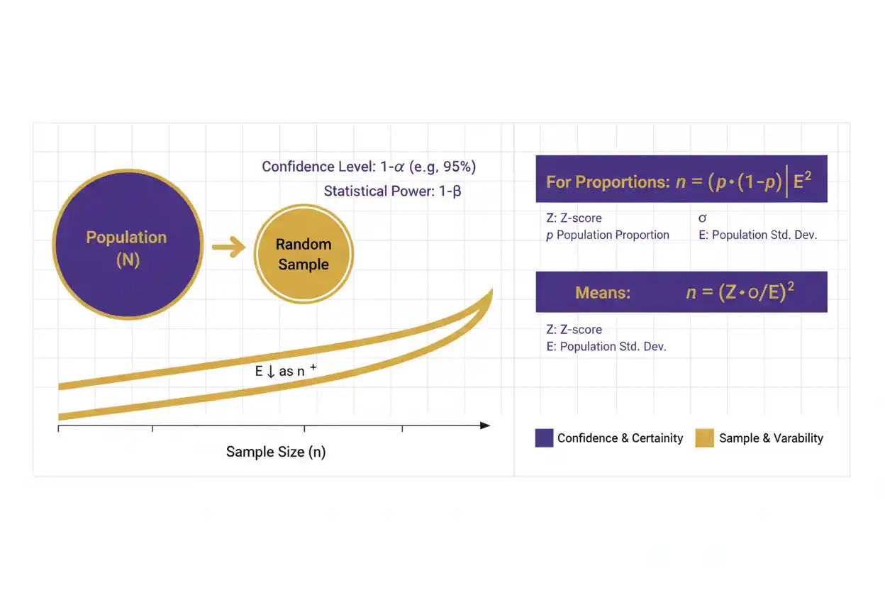
Sample size is the number of observations, participants, measurements, experimental units, or other independent units included in a statistical analysis, and it plays a central role in determining how precisely a sample can represent an unknown population quantity. A larger sample size generally reduces random sampling variability, narrows standard errors and confidence intervals, and increases the ability of a statistical test to detect a specified effect, but simply collecting more observations does not automatically eliminate bias, dependence, poor measurement, or an inappropriate study design. The appropriate sample size depends on the statistical objective: estimating a population proportion requires different inputs from estimating a mean, comparing two groups, fitting a regression model, estimating an extreme percentile, or designing a study for a specified level of statistical power. For a simple proportion estimate, sample size depends on the desired confidence level, margin of error, and anticipated population proportion; for a population mean, it depends on the desired precision and population standard deviation or a planning estimate of that standard deviation. Power-based calculations additionally require a significance level, target power, effect size, variability, and the exact statistical test or model. Because these quantities describe uncertainty rather than administrative convenience, sample size should be planned around the inferential or precision goal while also accounting for finite populations, clustering, unequal sampling, missing data, and expected attrition when those features apply.
Sample size belongs to the inferential foundations of core statistics and the wider Statistics & Probability framework. Its effect on uncertainty is best understood through sampling distributions, while the amount of information available from each observation depends partly on population variability summarized by measures such as standard deviation.
What Is Sample Size?
Sample size is commonly represented by:
n
and denotes the number of observations included in a sample.
For example, if a researcher measures the heights of:
250 people
then:
n = 250
If a study compares two independent groups containing:
100 observations each
the per-group sample sizes are:
n₁ = 100
n₂ = 100
and the total sample size is:
Ntotal = 200
The correct unit of sample size is the independent observational unit relevant to the analysis. Ten measurements taken from the same individual are not necessarily equivalent to ten independent people, because repeated observations from one unit can be correlated and therefore contain less independent information than ten unrelated units.
Why Sample Size Matters
Statistical estimates vary from sample to sample because a sample contains only part of the population information. If many independent random samples were collected from the same population, each sample would usually produce a somewhat different mean, proportion, regression slope, or other statistic.
Larger samples generally make those sample statistics more stable. Under common independent-sampling conditions, the standard error of many estimators decreases approximately in proportion to:
1/√n
This square-root relationship is fundamental. Doubling the sample does not halve ordinary sampling error; a much larger increase is required.
To cut a standard error approximately in half:
new n ≈ 4 × old n
because:
1/√(4n) = 1/(2√n)
The gain from increasing sample size therefore has diminishing returns.
Sample Size and Standard Error
For an independent sample mean, when the population standard deviation σ is known:
SE(x̄) = σ/√n
Suppose:
σ = 20
and:
n = 25
Then:
SE(x̄) = 20/5
= 4
If sample size increases to:
n = 100
then:
SE(x̄) = 20/10
= 2
The sample size increased by a factor of four, while the standard error decreased by a factor of two.
This relationship explains why very high precision can become expensive: each additional reduction in uncertainty requires progressively more observations.
Sample Size Formula for a Population Proportion
When the goal is to estimate a population proportion with a specified margin of error under a simple large-population random-sampling model, a common planning formula is:
n₀ = z*²p(1 − p)/E²
where:
- n₀ = initial required sample size
- z* = critical z-value for the chosen confidence level
- p = anticipated population proportion
- E = desired margin of error expressed as a proportion
The resulting n should normally be rounded up, because rounding downward would produce less precision than requested under the planning assumptions.
Sample Size Example for a Proportion
Suppose the desired confidence level is:
95%
with margin of error:
E = 0.05
and no reliable prior estimate of p is available.
A common conservative planning choice is:
p = 0.50
because:
p(1 − p)
is largest at 0.50, producing the largest required sample size under this formula.
For a 95% confidence level:
z* ≈ 1.96
Therefore:
n₀ = (1.96²)(0.50)(0.50)/(0.05²)
n₀ = (3.8416)(0.25)/0.0025
n₀ = 0.9604/0.0025
n₀ = 384.16
Round upward:
n = 385
Thus, under the simple planning assumptions, approximately 385 completed independent observations are required to estimate the proportion with a 5-percentage-point margin of error at the 95% confidence level.
Why p = 0.50 Is Conservative
The variance component for a binary outcome is:
p(1 − p)
Its maximum occurs at:
p = 0.50
because:
0.50(0.50) = 0.25
If instead:
p = 0.10
then:
p(1 − p) = 0.10(0.90)
= 0.09
which is much smaller.
Therefore, when no reliable planning estimate exists, p = 0.50 gives the largest sample size and protects against underestimating the variance within this simple proportion formula.
If credible prior evidence suggests a different p, using that value can produce a smaller planning requirement, but the result becomes dependent on the accuracy of the planning assumption.
Confidence Level and Sample Size
Higher confidence requires a larger critical value and therefore a larger sample size when all other inputs remain fixed.
Common two-sided standard-normal critical values are approximately:
| Confidence level | z* |
|---|---|
| 90% | 1.645 |
| 95% | 1.960 |
| 99% | 2.576 |
Because z* is squared in the sample size formula, increasing confidence can raise the required n substantially.
For p = 0.50 and E = 0.05, using 99% confidence gives:
n₀ = (2.576²)(0.25)/(0.05²)
≈ 663.6
so:
n = 664
compared with approximately:
385
for 95% confidence.
Greater confidence requires a wider interval at fixed n or, if the margin of error must remain unchanged, a larger sample.
Margin of Error and Sample Size
The desired margin of error appears in the denominator as:
E²
Therefore, reducing the margin of error has a strong effect on required sample size.
With 95% confidence and p = 0.50:
For:
E = 0.05
we need approximately:
n = 385
If the margin is cut in half to:
E = 0.025
the required sample becomes:
n₀ = (1.96²)(0.25)/(0.025²)
= 1,536.64
so:
n = 1,537
Halving the margin of error requires approximately four times as many observations.
This is the same square-root principle seen in standard errors.
Sample Size Formula for a Population Mean
When estimating a population mean with known or planning standard deviation σ and desired margin of error E, a common large-sample formula is:
n₀ = (z*σ/E)²
where:
- z* = confidence critical value
- σ = population standard deviation or planning estimate
- E = desired margin of error
The formula follows from the confidence-interval margin:
E = z*σ/√n
Solving for n gives:
√n = z*σ/E
and therefore:
n = (z*σ/E)²
Sample Size Example for a Mean
Suppose an analyst wants to estimate a population mean with:
95% confidence
a margin of error no greater than:
3 units
and an anticipated standard deviation:
σ = 12
Using:
z* = 1.96
we obtain:
n₀ = [1.96(12)/3]²
= (23.52/3)²
= 7.84²
= 61.4656
Round upward:
n = 62
Under those planning assumptions, at least 62 completed independent observations are required.
If the true standard deviation is larger than 12, the achieved margin of error will also be larger than planned unless the sample size is increased.
Why Standard Deviation Affects Sample Size
Greater population variability makes the population mean harder to estimate precisely.
Suppose two populations have the same mean but different standard deviations:
Population A: σ = 5
Population B: σ = 20
A sample of a given size will generally produce a much more variable sample mean from Population B because individual observations are more dispersed.
The mean-planning formula reflects this directly:
n ∝ σ²
If σ doubles while confidence and margin of error remain fixed, the required sample size increases approximately fourfold.
Reliable planning therefore benefits from pilot data, previous studies, or defensible external estimates of variability.
What If Standard Deviation Is Unknown?
In most real applications, the population standard deviation is unknown.
A planning analysis can use:
- a pilot-study estimate,
- historical data,
- a value from a comparable population,
- a conservative plausible upper estimate.
The final inferential procedure for a mean may use a t distribution rather than a z distribution, particularly when σ is estimated from the same sample.
For small planned samples, exact sample size calculations can therefore involve t critical values iteratively because the critical value itself depends on degrees of freedom.
The simple z-based formula remains a useful planning approximation, but its assumptions should be recognized.
Sample Size and Finite Populations
The basic formulas above behave as though the target population were extremely large relative to the sample. When sampling without replacement from a finite population and the sampling fraction is substantial, a finite population correction can reduce the number of independent units required for a fixed precision target.
If:
n₀
is the large-population sample requirement and the target population contains:
N
units, a common finite-population adjustment is:
n = n₀ / [1 + (n₀ − 1)/N]
Equivalently:
n = Nn₀/(N + n₀ − 1)
This formula applies within a simple random-sampling framework where the finite population correction is substantively appropriate.
Finite Population Example
Suppose the initial proportion calculation gives:
n₀ = 384.16
but the entire target population contains only:
N = 1,000
units.
Apply:
n = 384.16 / [1 + (384.16 − 1)/1000]
n = 384.16 / 1.38316
n ≈ 277.74
Round upward:
n = 278
Therefore, approximately 278 observations can provide the planned precision under this finite-population framework, rather than 385.
The reduction occurs because sampling 278 distinct units from a population of only 1,000 reveals a substantial fraction of the population directly.
Why Population Size Often Barely Matters
A common misconception is that a population of ten million must require dramatically more observations than a population of one hundred thousand.
Once the population is large relative to the sample, finite-population correction becomes negligible.
For example, a simple proportion estimate requiring around 385 observations under the large-population formula remains close to 385 whether the population contains:
100,000
or:
100,000,000
provided the sampling design and other assumptions are otherwise the same.
What matters most for sampling precision is usually:
- margin of error,
- confidence level,
- variability,
- study design,
rather than total population size once N is sufficiently large.
Sampling Fraction
The sampling fraction is:
f = n/N
When f is very small, finite population correction is close to 1 and can often be ignored for practical purposes.
When a large portion of the population is sampled without replacement, the correction becomes increasingly important.
A common finite-population standard-error factor is:
FPC = √[(N − n)/(N − 1)]
Multiplying a simple-random-sampling standard error by this factor reduces the uncertainty because the sample directly covers a substantial portion of the finite population.
The decision to use finite-population correction should follow the target population and sampling design rather than a universal percentage rule applied without context.
Sample Size and Sampling Distributions
The effect of sample size is fundamentally a statement about sampling distributions.
Suppose independent observations have population mean μ and variance σ².
The sample mean satisfies:
E(x̄) = μ
and:
Var(x̄) = σ²/n
Therefore:
SE(x̄) = σ/√n
As n increases, the sampling distribution of x̄ becomes more concentrated around μ.
This does not mean the raw observations themselves become less variable. The population standard deviation σ remains unchanged.
What becomes less variable is the estimator:
x̄
across repeated samples.
Sample Size and the Central Limit Theorem
Under suitable conditions, the central limit theorem states that the standardized sampling distribution of a sample mean or sum becomes increasingly close to normal as sample size grows.
This does not mean that a large raw data set itself becomes normally distributed.
If the population is strongly right-skewed, individual observations remain right-skewed regardless of n.
What can become approximately normal is the distribution of the sample mean across hypothetical repeated samples.
The sample size needed for an adequate approximation depends on population shape, tail behavior, dependence, and the statistic being considered. There is no universal rule that n = 30 automatically guarantees normality.
Sample Size and Probability
Sample size calculations are fundamentally statements about probability.
A 95% confidence procedure, for example, is designed around a repeated-sampling probability statement under the statistical model. A power calculation similarly asks for the probability of rejecting a null hypothesis when a specified alternative condition is true.
Therefore, choosing n is not simply an administrative decision about how much data would be convenient. It determines the probability behavior of estimators and tests under assumptions about variability, effect size, dependence, and design.
A mathematically precise sample size calculation can still fail to deliver its promised operating characteristics if those assumptions are badly wrong.
Sample Size and Statistical Power
Statistical power is:
Power = P(reject H₀ | specified alternative is true)
A common planning target is:
80%
or:
90%
although the appropriate target depends on the consequences and context of the study.
Power generally increases when:
sample size increases
because larger samples reduce the standard errors of estimated effects, making a fixed true departure from the null easier to distinguish from random variation.
Power also depends on effect size, significance level, outcome variability, study design, allocation ratio, and the particular statistical test.
There is therefore no universal “power sample size” formula that applies to every analysis.
Effect Size and Sample Size
Smaller effects require larger samples to detect reliably.
Suppose two studies use the same significance level, power, and outcome variability. Study A is designed to detect a large mean difference, while Study B seeks to detect a very small difference.
The distributions under the null and alternative are more strongly separated in Study A, so fewer observations may be needed.
Study B requires more precision to distinguish the small effect from random noise.
This is why a sample size calculation must specify what effect is considered important enough to detect. Without a target effect, a statement such as:
“We need 80% power”
is incomplete.
Two-Group Mean Comparison
For two independent groups of equal size, equal variance σ², a two-sided significance level α, and target power 1−β, a commonly used approximate planning formula for detecting mean difference Δ is:
n per group ≈ 2(zα/2 + zβ)²σ²/Δ²
where:
- zα/2 = two-sided critical value
- zβ = standard normal quantile corresponding to target power
- σ = common planning standard deviation
- Δ = mean difference to detect
The exact required n can differ when using t-based calculations, unequal variances, unequal allocation, repeated measures, covariate adjustment, or other designs.
Power-Based Example
Suppose a study wants:
α = 0.05
two-sided,
Power = 0.80
with:
σ = 10
and a target mean difference:
Δ = 5
Use approximately:
zα/2 = 1.96
and:
zβ = 0.842
Then:
n ≈ 2(1.96 + 0.842)²(10²)/(5²)
n ≈ 2(2.802²)(100)/25
n ≈ 62.8
Round upward:
n = 63 per group
Therefore, the approximate total sample size is:
126
before accounting for attrition or other design adjustments.
A more exact calculation can produce a slightly different result because the final test uses a t rather than a z reference distribution.
Statistical Significance Is Not the Planning Goal by Itself
A study should not be sized merely to “get p < 0.05.”
The sample size should relate to a scientifically or practically meaningful target effect and a specified probability of detecting that effect under a pre-defined testing procedure.
If the target effect is trivial but the sample is enormous, the study can achieve a very small p-value for a difference that has little practical consequence.
Conversely, a study that is too small can produce an imprecise estimate of an important effect.
Precision, effect magnitude, uncertainty, and practical relevance should therefore guide sample size planning together.
Sample Size and Regression
In a regression line, sample size affects uncertainty around the slope, intercept, fitted mean, and predictions, but no universal rule such as “10 observations per predictor” can guarantee adequate performance across all regression problems.
The amount of information available depends on:
- residual variability,
- predictor spread,
- predictor correlations,
- number of coefficients,
- effect sizes,
- model form,
- influential observations,
- intended inferential target.
For a simple regression slope:
SE(b₁) = s/√Sxx
under the classical model.
Increasing n can increase Sxx and stabilize the residual variance estimate, but the benefit depends on where the additional predictor observations occur.
A larger sample concentrated at nearly one x value can still contain little information about slope.
Sample Size and Predictor Range
Suppose one study measures x only between:
9.9 and 10.1
while another samples x throughout:
0 to 20.
Even with the same number of observations and residual noise, the second study can contain much more information about the regression slope because predictor variability is larger.
Sample size is therefore not the only determinant of precision.
Design matters.
A well-designed smaller study can sometimes provide more information about a target parameter than a larger but poorly distributed sample.
Multiple Regression
As the number of predictors and parameters increases, more observations are generally required to estimate coefficients reliably and evaluate predictive performance. However, the necessary sample size depends on the expected signal strength, predictor correlation, outcome distribution, regularization strategy, missingness, and the specific objective.
A model with five strong, weakly correlated predictors may require substantially less data than a model with five highly collinear predictors producing tiny effects. A regression used solely for prediction can also have different planning requirements from a model intended to estimate one coefficient with tight confidence limits.
Simple observation-per-variable rules should therefore be treated as rough heuristics rather than universal formulas.
Sample Size and Quartiles
Sample quartiles are estimates of population distributional positions, and their precision also depends on sample size.
With:
n = 8
only a few ordered observations determine Q₁ and Q₃, so changing one data point can noticeably alter the quartile estimates.
With:
n = 10,000
central sample quartiles generally become much more stable under representative independent sampling.
However, the exact uncertainty of a quantile depends on population density near that quantile. If relatively few population observations occur near Q₃, the estimated third quartile can remain less precise than a similarly sized sample from a distribution with high density around that point.
Extreme Percentiles Need Larger Samples
Estimating a median uses information near the middle of the distribution, where many observations often occur.
Estimating an extreme percentile such as:
P99.9
requires information about a very small tail region.
In a sample of:
n = 100
the expected number of observations above a true 99th percentile is only about:
1
and the sample contains essentially no direct empirical resolution for a 99.9th percentile.
Therefore, extreme-tail estimation often requires much larger samples or specialized tail models.
The necessary sample size depends on the percentile level, desired precision, and distributional assumptions.
Sample Size and Standard Deviation
The standard deviation affects many sample size formulas because it measures underlying dispersion.
For mean estimation:
n = (z*σ/E)²
so larger σ requires larger n.
For standardized effect sizes, a fixed raw difference becomes harder to detect when σ is large because the signal is smaller relative to the noise.
This relationship shows why sample size cannot be chosen sensibly from desired confidence and power alone.
The variability of the measurement is part of the information problem.
Design Effect
Simple sample size formulas usually assume something close to independent simple random sampling.
Clustered or otherwise correlated designs often contain less information per observation.
A common adjustment is:
n_complex ≈ DEFF × n_SRS
where:
DEFF
is the design effect relative to simple random sampling.
If:
DEFF = 2
a study may require roughly twice as many observations to achieve the variance that the simple-random-sample calculation anticipated.
The actual design effect should come from the sampling and correlation structure rather than being assumed arbitrarily.
Cluster Sampling
When observations are grouped into clusters, units from the same cluster can resemble one another.
A commonly used approximation for equal cluster size m and intracluster correlation ρ is:
DEFF ≈ 1 + (m − 1)ρ
Suppose:
m = 20
and:
ρ = 0.05
Then:
DEFF ≈ 1 + 19(0.05)
= 1.95
A simple-random-sample requirement of:
400
would then become approximately:
400(1.95)
= 780
observations before other adjustments.
The effective information can therefore be much smaller than the raw observation count suggests.
Effective Sample Size
A correlated or weighted data set can sometimes be summarized by an effective sample size: the number of independent equally weighted observations that would provide roughly comparable statistical information for a specified estimator.
For a rough design-effect interpretation:
neff ≈ n/DEFF
If:
n = 1,000
and:
DEFF = 2
then:
neff ≈ 500
This does not mean 500 records disappear physically. It means the estimator’s variance behaves roughly as though only 500 simple independent observations had been collected.
Effective sample size is method- and parameter-dependent, so one single value does not necessarily describe every statistic in a complex sample.
Unequal Weights
Survey or observational data can have unequal sampling weights.
When a small number of observations carry very large weights, the effective information can be lower than the raw n suggests because the estimate depends disproportionately on those observations.
A data set containing:
10,000 rows
does not automatically have the precision of 10,000 equally weighted independent observations.
Weight variability, clustering, stratification, and design must all be considered.
Sample size planning for complex surveys therefore generally requires more than inserting n into a simple random-sample formula.
Attrition
A study may require a certain number of completed observations but lose some units through withdrawal, missing follow-up, unusable measurements, or other forms of attrition.
If the required final sample is:
n_required
and the anticipated attrition proportion is:
r
a simple recruitment adjustment is:
n_recruit = n_required/(1 − r)
Suppose:
n_required = 385
and expected attrition is:
20%
Then:
n_recruit = 385/0.80
= 481.25
Round upward:
n_recruit = 482
Thus, approximately 482 units should be recruited to expect about 385 completed observations if the 20% attrition assumption is accurate.
Attrition Can Also Create Bias
Inflating recruitment protects the final count but does not solve every attrition problem.
If missingness is systematically related to outcomes, exposures, treatment effects, or other variables, the remaining sample can become biased even when the final n is numerically adequate.
For example, recruiting 1,000 participants and retaining 800 does not guarantee that the 800 are representative of the original target population.
Sample size addresses statistical information quantity.
Missing-data mechanisms determine whether the retained information remains valid for the intended inference.
Nonresponse
Survey sample planning must distinguish between:
invitations sent
and:
completed usable responses.
If the desired number of completed responses is 500 and the expected response rate is:
40%
then a simple planning calculation is:
invitations = 500/0.40
= 1,250
This adjustment addresses expected response volume.
It does not correct nonresponse bias if responders differ systematically from nonresponders.
A large response count from a biased recruitment or response process can still produce inaccurate population estimates.
Measurement Repetition vs Independent Sample Size
Suppose a laboratory measures one specimen 100 times.
The data contain:
100 measurements
but may contain only:
1 independent biological specimen.
The repeated measurements can improve precision about that specimen’s measurement process, but they do not necessarily provide the information of 100 independent specimens about population variability.
Similarly, repeated measurements from one person are usually correlated.
The effective sample size for a population-level parameter depends on the hierarchical structure, not simply the number of rows in a data file.
Pseudoreplication
Pseudoreplication occurs when non-independent observations are treated as though they were independent experimental replicates.
Suppose three experimental units are assigned to each treatment, and 100 measurements are taken from each unit.
The raw data contain:
300 measurements per treatment
but the independent treatment replication may still be only:
3 units
depending on the design and scientific question.
Treating all measurements as independent can severely underestimate standard errors and overstate precision.
Correct models account for the clustering or repeated-measures structure.
More Data Cannot Fix Systematic Bias
A huge sample can estimate the wrong target extremely precisely.
Suppose a survey asks only a nonrepresentative subgroup of the population.
Increasing the sample from:
1,000
to:
1,000,000
can make the sampling error tiny while leaving the selection bias unchanged.
The result becomes a very precise estimate of the subgroup’s behavior rather than an accurate estimate of the full target population.
Sample size controls random uncertainty under a design; it does not automatically repair poor sampling frames, confounding, measurement error, or nonresponse bias.
More Data Cannot Fix a Wrong Model
Similarly, a large sample does not make an inappropriate statistical model correct.
If observations are strongly dependent but analyzed as independent, or if a nonlinear relationship is forced into an unsuitable straight-line model, adding more data can produce extremely precise estimates of a misspecified relationship.
Large samples can actually make tiny model deviations statistically detectable while still leaving practical interpretation difficult.
Model adequacy and sample size should therefore be evaluated separately.
Very Small Samples
Small samples can produce unstable estimates, wide confidence intervals, and low power, particularly when the population is highly variable.
They are also more vulnerable to individual observations exerting substantial influence.
If:
n = 5
one observation represents:
20%
of the sample.
An unusual measurement can therefore alter the mean, standard deviation, regression slope, or quartiles considerably.
Small samples are not inherently invalid, but conclusions should reflect their limited information.
Large Samples
Large samples generally provide greater precision under suitable designs, but they create their own interpretive issues.
A tiny effect can become highly statistically significant when n is extremely large because standard errors become very small. Statistical significance can therefore diverge sharply from practical importance.
Large data sets can also contain many rare observations simply because there are more opportunities for rare events to appear.
Data quality, dependence, selection, and computational methodology remain important no matter how large n becomes.
Is n = 30 Always Enough?
No.
The statement:
“A sample size of 30 is always enough”
is not a valid general statistical rule.
Thirty observations may be more than adequate for one low-variance problem and grossly inadequate for another. Heavy-tailed distributions, rare outcomes, tiny effect sizes, clustered sampling, many regression parameters, or extreme percentile estimation can require substantially larger samples.
Conversely, some tightly controlled experiments with strong effects can produce useful information from fewer than 30 independent units.
Required sample size follows the statistical target and design rather than a universal cutoff.
Is 10% of the Population Enough?
Another unreliable rule is to sample a fixed percentage such as:
10% of the population.
For a population of one billion, 10% would mean one hundred million observations, vastly more than needed for many simple estimation problems.
For a population of twenty, 10% would mean only two observations, often far too few.
The relevant sample size depends on desired precision, variability, confidence, power, and design, with finite population size becoming especially relevant only when the sample represents a substantial portion of N.
Sample Size and Confidence Intervals
For many estimators, confidence interval width is approximately:
estimate ± critical value × standard error
Since standard error often declines as:
1/√n
larger sample size narrows the interval.
For a mean:
Margin ≈ z*σ/√n
For a proportion:
Margin ≈ z*√[p(1−p)/n]
under appropriate large-sample conditions.
This relationship is one of the clearest ways to interpret sample size: a larger n means a tighter range of estimates compatible with the data under the confidence procedure.
Precision vs Confidence
Suppose two studies estimate the same parameter.
Study A uses:
95% confidence
Study B uses:
99% confidence
If both have the same sample size and standard error, Study B will have a wider confidence interval because its critical value is larger.
To preserve the same interval width while increasing confidence, sample size must rise.
Thus, confidence and precision compete when n is fixed.
Sample size provides the additional information needed to improve one without sacrificing the other.
Sample Size and Rare Events
Rare-event studies can require very large samples even when the desired estimate seems simple.
Suppose an event occurs with probability:
p = 0.001
The expected number of events in n observations is:
np
With:
n = 100
the expected event count is only:
0.1
so most such samples will contain no events.
With:
n = 10,000
the expected count is:
10
which provides far more information.
When inference depends on observing enough rare outcomes, event counts rather than total n can become the practical limiting factor.
Sample Size and Subgroup Analysis
A study can have a large total sample while individual subgroups remain small.
Suppose:
n = 10,000
overall, but a subgroup of interest represents:
1%
of observations.
The expected subgroup size is only:
100
before missingness or additional stratification.
If the research requires precise subgroup-specific estimates, the overall sample should be planned to ensure adequate information within those groups.
A large total n does not guarantee precision for every subgroup or interaction.
Multiple Comparisons and Sample Size
If a study must support many comparisons, the required sample size can increase because significance thresholds may become more stringent or because power must be maintained across several planned tests.
Testing one pre-specified primary hypothesis at α = 0.05 is different from testing hundreds of outcomes while controlling a family-wise or false-discovery error criterion.
The correct calculation depends on the multiplicity procedure and inferential goal.
Sample size planning should therefore reflect the full planned analysis rather than only one isolated comparison when multiple testing materially affects the decision process.
One-Sided vs Two-Sided Tests
For the same α, effect size, variability, and target power, a justified one-sided test can require fewer observations than a two-sided test because the rejection region is concentrated in one pre-specified direction.
However, the direction must follow the scientific question before observing the data.
Choosing a one-sided test merely to reduce required sample size or obtain significance after seeing the result invalidates the intended error-rate interpretation.
The sample size calculation and eventual analysis should use the same test structure.
Unequal Group Allocation
Two-group studies do not always assign equal sample sizes.
Suppose one group is more expensive, scarce, or difficult to recruit.
Unequal allocation can be used, but for a fixed total sample and equal outcome variance, equal allocation is usually highly efficient for estimating a simple mean difference.
Large imbalance often reduces power unless justified by cost, variance differences, ethics, or other design considerations.
Sample size planning should therefore specify both total n and allocation ratio.
Pilot Studies
Pilot data can help estimate quantities needed for the final sample size calculation, such as:
- standard deviation,
- event rate,
- recruitment rate,
- intracluster correlation.
However, pilot estimates from very small samples can themselves be unstable.
Using an underestimated pilot standard deviation can produce an underpowered main study.
Therefore, planning often benefits from conservative estimates, uncertainty ranges, or sensitivity calculations showing how required n changes across plausible input values.
Sensitivity Analysis for Sample Size
A sample size calculation should rarely be treated as one unquestionable number when key inputs are uncertain.
Suppose σ could plausibly be:
8, 10, or 12
and the target margin of error is fixed.
Because:
n ∝ σ²
the resulting requirements can differ substantially.
Likewise, power calculations can be repeated for several plausible effect sizes.
Presenting this sensitivity helps decision-makers see which assumptions drive the required sample and whether recruitment capacity is compatible with the statistical objective.
Rounding Sample Size
When a formula produces:
n = 61.47
the requirement should ordinarily be rounded up:
n = 62
because 61 observations would provide slightly less information than the calculation requires.
If a study has multiple groups, rounding should generally be performed at the appropriate group level.
Further increases can then be added for anticipated attrition, nonresponse, clustering, or unusable observations.
Rounding downward solely for convenience undermines the planned precision or power, even if the numerical difference is small.
Common Sample Size Mistakes
A common mistake is choosing sample size from a universal rule such as n = 30 without considering the statistical objective, variance, effect size, or design. Another is assuming that larger population size always requires proportionally larger samples, even when the sampling fraction is tiny.
Another frequent error is calculating the number of completed observations needed but failing to inflate recruitment for expected attrition or nonresponse. Analysts can also count repeated measurements as independent observations, which makes the apparent n much larger than the actual independent information.
A further mistake is using p = 0.50 or a planning standard deviation without documenting that these are assumptions. The final precision depends on how closely those inputs match reality.
It is also incorrect to believe that a large sample guarantees unbiased or causal results. A large biased sample remains biased, and a large observational sample does not become randomized merely because n is high.
Finally, power calculations should use a meaningful target effect and the actual intended statistical test rather than being reverse-engineered simply to justify a convenient recruitment number.
How to Calculate Sample Size Step by Step
Begin by defining the statistical objective precisely. Decide whether the goal is estimating a proportion, estimating a mean, comparing groups, testing a hypothesis, fitting a regression model, or estimating a quantile, because each target has a different information structure.
Next choose the desired confidence level or significance level, precision or minimum meaningful effect, and target power when hypothesis testing is involved. Obtain a defensible planning estimate of variability, such as p for a proportion or σ for a mean, and determine whether the sampling design is approximately independent simple random sampling or requires clustering, weighting, or finite-population adjustments.
Calculate the initial n using the formula appropriate to the target, round upward, and then apply design effects or finite-population corrections where justified. Finally, inflate the result for anticipated attrition, nonresponse, missing data, or unusable measurements so that the expected completed analytical sample still reaches the statistical requirement.
Full Proportion Sample Size Example
Suppose a study wants to estimate a population proportion using:
95% confidence
with:
±4 percentage points
of margin of error.
No reliable planning estimate of p exists, so use:
p = 0.50
The formula is:
n₀ = z*²p(1−p)/E²
Substitute:
z* = 1.96
p = 0.50
E = 0.04
Then:
n₀ = (1.96²)(0.25)/(0.04²)
= 0.9604/0.0016
= 600.25
Round upward:
n = 601
Therefore, 601 completed independent observations are required under the large-population simple-random-sample assumptions.
Adding Attrition to the Example
Suppose expected unusable or missing observations are:
15%
The required recruitment becomes:
n_recruit = 601/(1 − 0.15)
= 601/0.85
≈ 707.06
Round upward:
n_recruit = 708
Thus, approximately 708 observations should be recruited to expect around 601 completed observations if the 15% loss assumption is accurate.
The statistical target remains 601 completed observations; 708 is the operational recruitment target.
Full Mean Sample Size Example
Suppose the objective is to estimate a population mean with:
99% confidence
and margin of error:
E = 2
Planning data suggest:
σ = 10
Use:
z* = 2.576
The required sample is:
n₀ = [2.576(10)/2]²
= (12.88)²
≈ 165.89
Round upward:
n = 166
If 10% attrition is expected:
n_recruit = 166/0.90
≈ 184.44
so:
n_recruit = 185
under the stated assumptions.
Interpreting the Final Sample Size
A calculated value such as:
n = 385
does not mean that 384 observations are statistically worthless or that observation 385 creates a magical boundary between failure and validity.
The result is a planning threshold derived from specific inputs and an operating criterion. Slightly fewer observations produce slightly less precision or power; slightly more produce slightly greater precision.
The important distinction is between:
meeting the planned statistical performance
and:
treating a threshold as an absolute law.
If the achieved sample differs from the target, the final analysis should report the actual n and quantify the uncertainty actually obtained.
How to Report Sample Size
A transparent sample size statement should explain the assumptions that generated the target rather than report only the final number.
For example:
“The planned sample size was 385 completed observations, based on a two-sided 95% confidence level, a ±5 percentage-point margin of error, and the conservative planning proportion p = 0.50 under simple random sampling.”
If attrition was included:
“The recruitment target was increased to 482 to allow for an anticipated 20% loss.”
For a power analysis, report the significance level, target power, minimum effect, variance assumption, group allocation, and test structure.
This makes the calculation reproducible and clarifies what statistical performance the planned sample was intended to provide.
Frequently Asked Questions About Sample Size
What is sample size?
Sample size is the number of observations or independent experimental units included in a statistical sample and is commonly represented by n.
Why is sample size important?
It affects sampling variability, standard errors, confidence-interval width, statistical power, and the stability of many estimated statistics.
Does a larger sample always give a better estimate?
It usually reduces random sampling error under an appropriate design, but it does not automatically correct bias, dependence, measurement problems, or model misspecification.
What is the sample size formula for a proportion?
A common large-population planning formula is:
n₀ = z*²p(1−p)/E²
What should I use for p if it is unknown?
A common conservative choice is:
p = 0.50
because p(1−p) is largest at 0.50.
What is the sample size formula for a mean?
A common planning formula is:
n₀ = (z*σ/E)²
Why is sample size rounded upward?
Rounding downward would provide slightly less precision or power than the calculation requires.
How many observations are needed for 95% confidence and a 5% margin of error?
For a simple large-population proportion estimate using p = 0.50:
n ≈ 385
before design or attrition adjustments.
Does a population of millions require millions of observations?
Not for many simple random-sampling estimation problems. Once the population is large relative to n, total population size has little effect on the required sample for a fixed confidence and margin of error.
When does finite population size matter?
It matters when sampling without replacement and the sample is a substantial fraction of the finite target population.
What is the finite population sample size formula?
One common correction is:
n = n₀/[1 + (n₀−1)/N]
What is a finite population correction?
A common standard-error factor is:
√[(N−n)/(N−1)]
which reflects the extra information gained when a substantial portion of the finite population is sampled without replacement.
How does margin of error affect sample size?
Required n is approximately proportional to:
1/E²
so halving the margin of error requires roughly four times the sample.
How does confidence level affect sample size?
Higher confidence uses a larger critical value, increasing the required sample if the margin of error is held fixed.
How does standard deviation affect sample size?
For mean estimation:
n ∝ σ²
so greater population variability requires more observations for the same precision.
What is statistical power?
Power is:
P(reject H₀ | a specified alternative is true)
and usually increases as sample size increases.
Is 80% power always required?
No. It is a common planning target, but the appropriate power depends on the consequences and objectives of the study.
What is effect size?
Effect size describes the magnitude of the difference, association, or departure from the null that the study aims to estimate or detect.
Why do smaller effects require larger samples?
Small effects are harder to distinguish from random variation, so more observations are generally required to estimate them precisely or detect them with high power.
Does n = 30 guarantee a sufficient sample?
No. Required sample size depends on the statistical target, variability, design, distribution, effect size, and desired precision or power.
Is sampling 10% of a population a good rule?
No. A fixed population percentage can be far too large for huge populations and far too small for tiny ones.
What is design effect?
Design effect compares the variance under a complex sampling design with the variance under an equivalent simple random sample.
How does clustering affect sample size?
Positive within-cluster correlation reduces the amount of independent information, often requiring a larger raw sample.
What is a common cluster design-effect approximation?
For equal cluster size m and intracluster correlation ρ:
DEFF ≈ 1 + (m−1)ρ
What is effective sample size?
It is the approximate number of independent equally weighted observations that would provide comparable statistical information for a specified estimator.
Is the number of rows in a data set always the sample size?
Not necessarily. Repeated measurements, clustering, and dependence can make the number of independent units much smaller than the number of recorded rows.
What is pseudoreplication?
It is the error of treating correlated or repeated measurements as independent replicates, which can exaggerate the apparent sample size and understate uncertainty.
How should attrition be handled in sample size planning?
If r is the expected loss proportion:
n_recruit = n_required/(1−r)
Does increasing recruitment solve attrition bias?
No. It can preserve the final number of observations but does not remove systematic bias if the units lost differ meaningfully from those retained.
Can a huge sample still be biased?
Yes. Increasing n reduces random sampling error but does not automatically eliminate selection bias, nonresponse bias, confounding, or measurement error.
How does sample size affect regression?
Larger informative samples can improve precision of regression coefficients and predictions, but predictor spread, noise, multicollinearity, model complexity, and dependence also matter.
Is there a universal number of observations per regression predictor?
No. Such rules are rough heuristics and cannot replace planning based on effect sizes, variability, predictor structure, objectives, and validation requirements.
How does sample size affect quartiles?
Larger samples generally produce more stable estimates of population quartiles, while small-sample quartiles can vary substantially and depend more visibly on calculation convention.
Why do extreme percentiles require larger samples?
Extreme percentiles depend on small tail fractions, so relatively few observations inform them unless n is large.
Does the central limit theorem say n = 30 is enough?
No. The quality of a normal approximation depends on the population distribution, statistic, dependence structure, and required accuracy.
How can I make a confidence interval narrower?
Other factors being fixed, increase sample size or accept a lower confidence level. Reducing underlying variability can also improve precision when study design permits it.
If I double the sample size, does the margin of error halve?
Not generally. Since ordinary standard errors scale approximately as 1/√n, doubling n reduces them by a factor of:
1/√2 ≈ 0.707
not by one-half.
How much must sample size increase to halve the standard error?
Approximately fourfold under the usual 1/√n relationship.
What should a sample size report include?
It should state the statistical objective, confidence or significance level, desired precision or target effect, power when relevant, variability assumptions, allocation or sampling design, and adjustments for attrition or clustering.
What is the most important rule for choosing sample size?
Choose sample size from the statistical question, desired precision or power, variability, and actual study design rather than from a universal numerical rule or a convenient recruitment target.




