


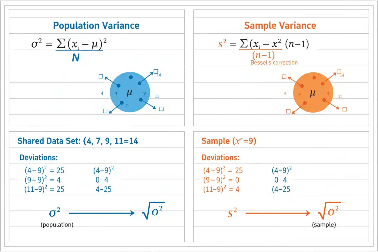
Variance measures how widely numerical values are dispersed around their arithmetic mean by averaging squared deviations from that mean, and the distinction between population variance and sample variance determines which denominator should be used. When every value in the population of interest is available and the goal is simply to describe that population, population variance divides the total squared deviation by N. When observations form a sample used to estimate variability in a larger population, the conventional sample variance divides by n − 1 instead, a correction that compensates for the tendency of squared deviations around the estimated sample mean to underestimate the unknown population variance. This difference is fundamental rather than cosmetic because N and n − 1 represent different statistical purposes: one describes a known finite set, while the other creates an unbiased estimator of σ² under standard random-sampling assumptions. Variance is expressed in squared measurement units, which can make it less intuitive than standard deviation, but its algebraic properties make it indispensable in probability, sampling theory, regression, hypothesis testing, portfolio analysis, error propagation, and many other statistical calculations.
Variance is a foundational concept in statistics basics and within the broader core statistics framework. It is directly related to standard deviation, while inferential procedures such as the t-test and z-test rely on variance or standard-error quantities to compare observed effects with expected sampling variability.
What Is Variance?
Variance is a measure of dispersion around the mean.
If observations are tightly clustered near their mean, variance is small. If observations are spread far from the mean, variance is larger.
The basic idea is:
Variance = average squared deviation from the mean
The word squared is essential. If ordinary deviations were added directly, positive and negative differences would cancel.
For any data set:
Σ(xᵢ − mean) = 0
when the mean is the arithmetic mean.
Squaring each deviation prevents cancellation:
(xᵢ − mean)² ≥ 0
and gives larger deviations greater influence on the final result.
Population Variance Formula
For a population containing N values, population variance is:
σ² = Σ(xᵢ − μ)² / N
where:
- σ² = population variance
- xᵢ = individual population value
- μ = population mean
- N = population size
Use this formula when the observations represent the entire population being described rather than a sample being used to estimate a larger population.
The population mean is:
μ = Σxᵢ / N
Once μ is known, each value’s deviation from μ is squared, the squared deviations are summed, and the total is divided by N.
Sample Variance Formula
For a sample containing n observations, the conventional sample variance is:
s² = Σ(xᵢ − x̄)² / (n − 1)
where:
- s² = sample variance
- xᵢ = sample observation
- x̄ = sample mean
- n = sample size
The sample mean is:
x̄ = Σxᵢ / n
The denominator is:
n − 1
rather than n because x̄ is itself estimated from the same sample.
This adjustment is called Bessel’s correction.
Population vs Sample Variance
The central comparison is:
Population variance: σ² = Σ(xᵢ − μ)² / N
Sample variance: s² = Σ(xᵢ − x̄)² / (n − 1)
The formulas look almost identical, but their interpretation is different.
Population variance describes the actual variability of the complete population under consideration.
Sample variance estimates an unknown population variance using sample data.
If the same five observations are treated first as the complete population and then as a sample from a larger population, the squared deviations can be identical while the final variance differs because the denominator changes.
Population Variance Example
Suppose the entire population is:
2, 4, 6, 8, 10
There are:
N = 5
values.
First calculate the population mean:
μ = (2 + 4 + 6 + 8 + 10)/5
μ = 30/5
μ = 6
Now calculate deviations:
2 − 6 = −4
4 − 6 = −2
6 − 6 = 0
8 − 6 = 2
10 − 6 = 4
Square them:
16, 4, 0, 4, 16
The sum of squared deviations is:
40
Population variance is:
σ² = 40/5
σ² = 8
Therefore, the variance of this complete population is:
8
Sample Variance Example
Now suppose the same values:
2, 4, 6, 8, 10
are a sample from a larger population.
The sample mean is still:
x̄ = 6
and the squared deviations still sum to:
40
However, the sample variance is:
s² = 40/(5 − 1)
s² = 40/4
s² = 10
Thus:
Sample variance = 10
The difference between:
8
and:
10
does not come from different data. It comes from the different statistical purpose of the calculation.
Why Does Sample Variance Use n − 1?
The sample mean x̄ is calculated from the observations themselves and tends to lie closer to those observations than the unknown population mean μ would, on average.
As a result:
Σ(xᵢ − x̄)²
tends to be smaller than the squared-deviation total that would be obtained around the true μ.
If this total were divided by n, the resulting estimator would systematically underestimate σ².
Dividing by:
n − 1
corrects that downward bias under independent sampling from a population with finite variance.
Mathematically:
E(s²) = σ²
when s² uses the n − 1 denominator under the usual assumptions.
Degrees of Freedom
The phrase degrees of freedom helps explain the n − 1 denominator.
Once the sample mean x̄ has been calculated, the deviations satisfy:
Σ(xᵢ − x̄) = 0
Suppose a sample has five observations. If four deviations from the mean are known, the fifth deviation is automatically determined because the total must equal zero.
Therefore, only:
n − 1
deviations can vary freely.
The sample variance uses those n − 1 degrees of freedom when estimating the unknown population variance.
Bessel’s Correction
Bessel’s correction refers to replacing n with:
n − 1
when calculating the conventional sample variance.
Without the correction:
Biased variance estimate = Σ(xᵢ − x̄)²/n
With the correction:
s² = Σ(xᵢ − x̄)²/(n − 1)
The corrected version is unbiased for σ² under the standard independent-identically-distributed model.
This does not mean the corrected sample variance equals the population variance in every sample. Individual samples can overestimate or underestimate σ².
Unbiasedness means that across repeated samples:
average s² = σ²
in expectation.
Variance vs Standard Deviation
Variance and standard deviation contain closely related information.
Standard deviation is the square root of variance:
σ = √σ²
for a population, and:
s = √s²
for a sample.
Conversely:
σ² = σ × σ
s² = s × s
The main interpretive difference concerns units.
If a variable is measured in:
meters
variance is measured in:
meters²
while standard deviation is measured in:
meters.
Standard deviation is usually more intuitive for describing spread, while variance is especially convenient in mathematical derivations.
Why Variance Uses Squared Units
Suppose observations are measured in kilograms.
A deviation:
x − μ
is also measured in kilograms.
After squaring:
(x − μ)²
the unit becomes:
kilograms²
Averaging these squared deviations leaves variance in kilograms².
Taking the square root returns to kilograms:
Standard deviation = √Variance
The squared units are not an error. They arise directly from the definition of variance.
Step-by-Step Variance Example
Consider the sample:
5, 7, 8, 10, 15
First calculate the mean:
x̄ = (5 + 7 + 8 + 10 + 15)/5
x̄ = 45/5
x̄ = 9
Now calculate deviations and squared deviations:
| x | x − 9 | (x − 9)² |
|---|---|---|
| 5 | −4 | 16 |
| 7 | −2 | 4 |
| 8 | −1 | 1 |
| 10 | 1 | 1 |
| 15 | 6 | 36 |
The squared deviations sum to:
16 + 4 + 1 + 1 + 36
= 58
Since the observations are treated as a sample:
s² = 58/(5 − 1)
s² = 58/4
s² = 14.5
Therefore:
Sample variance = 14.5
and sample standard deviation is:
s = √14.5
s ≈ 3.808
Interpreting Variance
Variance should primarily be interpreted as a measure of dispersion rather than as an average ordinary distance from the mean.
In the previous sample:
s² = 14.5
does not mean observations are typically:
14.5 units
from the mean.
The value is measured in squared units.
For direct distance interpretation, use:
s ≈ 3.81
the corresponding standard deviation.
Variance is especially valuable because squared deviations have powerful mathematical properties, including additivity under independence and simple behavior under linear transformations.
Zero Variance
Variance equals zero when every observation is identical.
Suppose:
12, 12, 12, 12
The mean is:
12
Every deviation is:
0
and every squared deviation is:
0
Therefore:
Variance = 0
A zero variance means the variable has no observed or population dispersion.
It does not mean the mean is zero.
Variance Cannot Be Negative
Every squared deviation satisfies:
(xᵢ − μ)² ≥ 0
or:
(xᵢ − x̄)² ≥ 0
Therefore, their sum is nonnegative, and dividing by a positive denominator preserves that property.
Thus:
Variance ≥ 0
A negative calculated variance indicates an arithmetic, numerical, or formula error.
In floating-point computing, extremely tiny negative values can occasionally appear from numerical roundoff in unstable algorithms, but the true mathematical variance cannot be negative.
Larger Variance Means Greater Dispersion
Consider:
A = 48, 49, 50, 51, 52
and:
B = 10, 30, 50, 70, 90
Both populations have:
μ = 50
For A, the squared deviations are:
4, 1, 0, 1, 4
so:
σA² = 10/5
= 2
For B, squared deviations are:
1600, 400, 0, 400, 1600
so:
σB² = 4000/5
= 800
Therefore, B has dramatically greater variance even though both populations share the same mean.
Center and spread describe different characteristics.
Variance and Outliers
Variance is highly sensitive to extreme values because deviations are squared.
Suppose the population is:
8, 9, 10, 11, 12
Its mean is:
10
and population variance is:
(4 + 1 + 0 + 1 + 4)/5
= 2
Now replace 12 with 100:
8, 9, 10, 11, 100
The mean becomes:
27.6
and the squared deviations become much larger.
The population variance rises to approximately:
1311.44
One extreme observation can therefore change variance dramatically.
Variance is not a robust measure of spread.
Variance vs Interquartile Range
The interquartile range focuses on the middle 50% of ordered data:
IQR = Q₃ − Q₁
Variance uses every observation and squares each deviation from the mean.
As a result, variance responds strongly to extreme observations, while the IQR is much more resistant.
For approximately symmetric distributions without problematic extremes, mean and variance can provide efficient summaries.
For heavily skewed data, median and IQR can often describe central location and spread more robustly.
Neither approach is universally correct for every distribution.
Variance Shortcut Formula
Population variance can be rewritten as:
σ² = (Σxᵢ²/N) − μ²
This follows from the identity:
Var(X) = E(X²) − [E(X)]²
For a finite population:
E(X²) = Σxᵢ²/N
and:
E(X) = μ
Therefore:
σ² = E(X²) − μ²
This shortcut can make hand calculations easier, although centered formulas are often numerically safer in software when values are very large and variance is relatively small.
Sample Variance Shortcut Formula
The sample variance can be calculated as:
s² = [Σxᵢ² − n x̄²]/(n − 1)
An equivalent form is:
s² = [Σxᵢ² − (Σxᵢ)²/n]/(n − 1)
Return to:
5, 7, 8, 10, 15
We have:
Σx = 45
and:
Σx² = 25 + 49 + 64 + 100 + 225
Σx² = 463
Then:
s² = [463 − 45²/5]/4
= [463 − 2025/5]/4
= (463 − 405)/4
= 58/4
= 14.5
This matches the direct deviation method.
Variance as Expected Squared Deviation
For a random variable X with finite second moment:
Var(X) = E[(X − μ)²]
where:
μ = E(X)
This population-probability definition generalizes variance beyond finite lists of observations.
Expanding the square gives:
Var(X) = E(X²) − [E(X)]²
This identity is widely useful in probability calculations.
It also shows that variance depends on the first two moments of the distribution.
Variance Under Addition of a Constant
Suppose:
Y = X + c
Then:
Var(Y) = Var(X)
Adding a constant shifts every value and the mean by the same amount, so distances from the mean remain unchanged.
For example:
1, 2, 3
and:
101, 102, 103
have the same variance.
The distributions are located differently, but their spread is identical.
Variance is therefore unaffected by changes in origin.
Variance Under Multiplication
Suppose:
Y = aX
Then:
Var(Y) = a²Var(X)
If every observation is doubled:
a = 2
then variance is multiplied by:
2² = 4
If every observation is divided by 10:
a = 0.1
variance is multiplied by:
0.1² = 0.01
For a general linear transformation:
Y = aX + b
the variance is:
Var(Y) = a²Var(X)
The additive constant b has no effect on spread.
Example of Scaling Variance
Suppose X has:
Var(X) = 9
and define:
Y = 5X + 100
Then:
Var(Y) = 5²(9)
= 25(9)
= 225
The corresponding standard deviations are:
SD(X) = 3
and:
SD(Y) = 15
Notice:
15 = 5(3)
while:
225 = 25(9)
Standard deviation scales by |a|, while variance scales by a².
Variance of a Sum
For any two random variables X and Y with finite variances:
Var(X + Y) = Var(X) + Var(Y) + 2Cov(X,Y)
If X and Y are independent:
Cov(X,Y) = 0
so:
Var(X + Y) = Var(X) + Var(Y)
This additivity is one of the most important reasons variance is mathematically useful.
Standard deviations do not generally add directly.
If two independent variables have standard deviations 3 and 4, their sum has variance:
3² + 4² = 25
and standard deviation:
√25 = 5
not:
3 + 4 = 7
Variance of a Difference
For:
X − Y
the general rule is:
Var(X − Y) = Var(X) + Var(Y) − 2Cov(X,Y)
If X and Y are independent:
Cov(X,Y) = 0
so:
Var(X − Y) = Var(X) + Var(Y)
Even though the random variables are subtracted, their independent variances add.
This happens because:
Var(−Y) = Var(Y)
Changing the sign of every Y value does not change its spread.
Variance and Covariance
Covariance measures how two variables vary together.
The relationship:
Var(X + Y) = Var(X) + Var(Y) + 2Cov(X,Y)
shows why dependence matters.
If covariance is positive, X and Y tend to move together, increasing the variance of their sum.
If covariance is negative, their movements partly offset one another, reducing the variance of the sum.
If covariance is zero, the variance of the sum equals the sum of individual variances.
Independence implies zero covariance when the necessary moments exist, although zero covariance does not generally imply independence.
Variance of the Sample Mean
Suppose:
X₁, X₂, …, Xₙ
are independent observations with common variance:
σ²
The sample mean is:
X̄ = (X₁ + … + Xₙ)/n
The variance of the sum is:
nσ²
Under independence.
Scaling by 1/n gives:
Var(X̄) = (1/n²)(nσ²)
Therefore:
Var(X̄) = σ²/n
Its standard deviation is:
SD(X̄) = σ/√n
which is the standard error of the sample mean.
This connects population variance directly with sampling uncertainty.
Sample Size and Variance of an Estimator
Because:
Var(X̄) = σ²/n
increasing n reduces the variance of the sample mean.
If sample size quadruples:
n → 4n
then:
Var(X̄) → σ²/(4n)
so the sampling variance becomes one-quarter as large.
The standard error becomes one-half as large because it is the square root of variance.
This distinction explains why variance shrinks with:
1/n
while standard error shrinks with:
1/√n
for the sample mean.
Variance of a Bernoulli Variable
A Bernoulli random variable has:
X = 1
with probability p and:
X = 0
with probability:
1 − p
Its mean is:
E(X) = p
and variance is:
Var(X) = p(1 − p)
The variance is largest when:
p = 0.5
giving:
Var(X) = 0.25
As p approaches 0 or 1, the outcome becomes increasingly predictable and variance approaches zero.
This formula is central to sample-proportion standard errors.
Variance of a Binomial Variable
If:
X ~ Binomial(n,p)
then:
E(X) = np
and:
Var(X) = np(1 − p)
The standard deviation is:
√[np(1 − p)]
This result follows because a binomial count can be represented as the sum of n independent Bernoulli variables, each with variance:
p(1 − p)
Independent variances add, yielding:
n × p(1 − p)
Variance of a Poisson Variable
If:
X ~ Poisson(λ)
then:
E(X) = λ
and:
Var(X) = λ
Thus, the Poisson model has the characteristic property:
Mean = Variance
Its standard deviation is:
√λ
This equality is a population-model property.
A finite random sample from a Poisson population will not generally have sample mean exactly equal to sample variance.
Large systematic discrepancies between sample mean and variance can, however, provide clues that a simple Poisson model may be inadequate.
Variance of a Normal Distribution
If:
X ~ N(μ,σ²)
the second parameter:
σ²
is the variance.
Thus:
Mean = μ
Variance = σ²
Standard deviation = σ
Changing μ shifts the normal distribution left or right without changing its spread.
Changing σ² changes its dispersion around μ.
Because normal distributions are completely characterized by μ and σ², variance plays a particularly central role in normal-theory inference.
Standardizing Removes Variance Scale
Define the z-score transformation:
Z = (X − μ)/σ
provided:
σ > 0
Then:
E(Z) = 0
and:
Var(Z) = 1
To verify:
Var[(X − μ)/σ]
= (1/σ²)Var(X)
= σ²/σ²
= 1
Thus, standardization produces a variable with unit variance.
This does not make the distribution normal unless X was normal to begin with; it only changes location and scale.
Variance and the z-Test
A z-test for a population mean with known σ uses:
z = (x̄ − μ₀)/(σ/√n)
The denominator follows from:
Var(X̄) = σ²/n
and therefore:
SD(X̄) = σ/√n
The z statistic measures the sample mean’s distance from the null mean in units of its sampling standard deviation.
Variance is therefore embedded directly in the test even though the final formula is usually written using σ rather than σ².
Variance and the t-Test
When population variance is unknown, the t-test replaces σ² with information estimated from the sample.
For a one-sample t-test:
t = (x̄ − μ₀)/(s/√n)
where:
s² = Σ(xᵢ − x̄)²/(n − 1)
The use of estimated variance introduces additional uncertainty, which is why the statistic follows a t distribution rather than a standard normal distribution under the classical normal model.
Thus, the n − 1 correction in sample variance is directly connected to one of the most widely used inferential tests.
Sampling Distribution of Sample Variance
Suppose:
X₁,…,Xₙ
are independent observations from:
N(μ,σ²)
Then the conventional sample variance satisfies:
(n − 1)S²/σ² ~ χ²₍ₙ₋₁₎
This exact result shows that sample variance itself is random.
Different samples from the same normal population produce different S² values.
The chi-square sampling distribution forms the basis of classical confidence intervals and hypothesis tests for a normal population variance.
Confidence Interval for a Normal Population Variance
Because:
(n − 1)S²/σ²
has a chi-square distribution under normal sampling, a confidence interval for σ² can be constructed using chi-square critical values.
A two-sided interval takes the form:
[(n − 1)s²/χ²_upper, (n − 1)s²/χ²_lower]
where the chi-square critical values correspond to the required tail probabilities and:
df = n − 1
The interval is usually asymmetric because the chi-square distribution is right-skewed.
Taking square roots of the interval endpoints produces a corresponding confidence interval for σ.
Sample Variance Is Unbiased, but Sample Standard Deviation Is Not Exactly Unbiased
The conventional sample variance satisfies:
E(S²) = σ²
under standard conditions.
However:
E(√S²) ≠ √E(S²)
in general.
Therefore, although S² is unbiased for σ²:
S = √S²
is not exactly unbiased for σ.
Its bias is usually downward and becomes smaller as sample size increases.
This is an important example of a broader principle: applying a nonlinear transformation to an unbiased estimator does not generally preserve unbiasedness.
Mean Squared Error
For an estimator θ̂ of a parameter θ:
MSE(θ̂) = E[(θ̂ − θ)²]
The mean squared error decomposes into:
MSE(θ̂) = Var(θ̂) + [Bias(θ̂)]²
This formula shows why variance is central not only for describing raw data but also for evaluating estimators.
An estimator with low bias can still perform poorly if its variance is very large.
Conversely, a slightly biased estimator can sometimes have lower MSE if its variance is substantially smaller.
Statistical performance often involves balancing both components.
Within-Group and Between-Group Variance
When data contain groups, overall variation can often be separated conceptually into:
variation within groups
and:
variation between group means.
Suppose two groups are each tightly clustered internally but their means differ substantially.
Each group can have small within-group variance while the combined data have large overall variance.
This distinction underlies analysis of variance and many hierarchical statistical models.
A large total variance does not identify whether spread arises within units, between subgroups, or from both sources.
Pooled Variance
When two independent populations are assumed to have a common variance, their sample variances can be pooled:
sₚ² = [(n₁ − 1)s₁² + (n₂ − 1)s₂²] / (n₁ + n₂ − 2)
This is a degrees-of-freedom-weighted average of the two sample variances.
Suppose:
n₁ = 10, s₁² = 16
n₂ = 20, s₂² = 25
Then:
sₚ² = [(9)(16) + (19)(25)]/28
= (144 + 475)/28
= 619/28
≈ 22.107
The pooled standard deviation is:
sₚ ≈ √22.107
≈ 4.702
Pooling is appropriate only when the common-variance assumption is justified.
Variance and Measurement Precision
Low variance among repeated measurements can indicate high repeatability.
Suppose a device repeatedly measures the same object as:
100.1, 100.0, 99.9, 100.1
These measurements have very small variance.
However, low variance does not establish accuracy.
If the true value is:
95
then the device is consistently wrong despite being highly precise.
Variance measures dispersion.
Bias measures systematic displacement from the target.
Both matter when evaluating measurement quality.
Variance and Scale
Variance depends strongly on measurement scale because multiplying values by a changes variance by a².
Suppose distances measured in meters have:
Variance = 4 m²
Converting meters to centimeters multiplies each measurement by:
100
Therefore, variance becomes:
100² × 4
= 40,000 cm²
The numerical variance changes dramatically even though the physical variability is unchanged.
This scale dependence is why variance should not usually be compared directly across unrelated measurement units.
Comparing Variance Across Variables
Suppose Variable A has:
Variance = 100
and Variable B has:
Variance = 25
It is not automatically meaningful to say A is “four times more variable.”
The interpretation depends on:
- units,
- scale,
- mean levels,
- distribution shape,
- measurement meaning.
If A and B use the same measurement scale and comparable contexts, the comparison can be meaningful.
Across different units, standardized or relative measures may be more appropriate.
Variance and Skewed Data
Variance can be calculated for skewed data whenever the relevant second moment exists.
However, squared deviations make it particularly sensitive to long tails.
Suppose most values lie between:
10 and 20
but a few values exceed:
1,000.
Those rare extremes can dominate the variance.
Reporting the median and interquartile range alongside variance or standard deviation can provide a more complete description.
The appropriateness of variance as the main spread measure therefore depends on distribution shape and analytical purpose.
Infinite or Undefined Variance
Not every probability distribution has finite variance.
Some heavy-tailed distributions assign enough probability to extreme values that:
E[(X − μ)²]
does not exist as a finite number.
The Cauchy distribution is a classic example: it does not have a finite population mean or variance.
In such cases, standard methods relying on σ² can fail or become conceptually inappropriate.
Observing a finite sample variance does not prove that the underlying theoretical population variance exists, because every finite numerical sample produces some finite arithmetic value unless computation overflows.
Variance and Missing Data
Variance calculations should use the observations legitimately included in the analysis.
Replacing missing values automatically with zero changes:
- the mean,
- deviations,
- squared deviations,
- variance.
This can produce severe distortion unless zero genuinely represents the missing quantity.
Simply dropping missing observations can also create bias if missingness is systematically related to the variable.
Data-quality decisions should therefore precede mechanical variance calculation.
Variance With Frequency Data
If values occur with frequencies fᵢ, population variance can be calculated as:
σ² = Σfᵢ(xᵢ − μ)² / N
where:
N = Σfᵢ
and:
μ = Σfᵢxᵢ / N
This avoids expanding every repeated value individually.
For a probability distribution, frequencies are replaced by probabilities:
Var(X) = Σ(x − μ)²P(X=x)
for a discrete random variable.
Frequency-weighted and probability-weighted variance use the same squared-deviation principle.
Weighted Variance
When observations carry unequal statistical weights, variance calculations become more complicated because the correct denominator depends on what the weights represent.
Weights might correspond to:
- frequencies,
- survey sampling weights,
- reliability weights,
- analytic importance.
A simple weighted population mean can be written:
μw = Σwᵢxᵢ / Σwᵢ
and a descriptive weighted population variance as:
σw² = Σwᵢ(xᵢ − μw)² / Σwᵢ
However, unbiased sample-variance corrections for arbitrary weights are not obtained merely by replacing n with:
Σwᵢ − 1
in every setting.
The weighting design determines the appropriate estimator.
Common Variance Mistakes
A common mistake is using N when the task requires estimating an unknown population variance from sample data, or using n − 1 when the observed values are being treated as the complete population being described. The denominator depends on the statistical role of the data.
Another error is forgetting to square deviations. Ordinary deviations around the arithmetic mean sum to zero and therefore cannot directly measure dispersion.
Another common mistake is calling variance an “average distance” from the mean. It is an average squared distance under the population formula, not an ordinary distance in the original units.
Analysts also sometimes assume variance and standard deviation can be used interchangeably without considering their units.
Another mistake is adding standard deviations instead of variances when independent random quantities are combined.
It is also incorrect to assume that sample variance must equal population variance merely because it is unbiased. Unbiasedness is a repeated-sampling property, not equality in each sample.
Finally, a large variance should not automatically be interpreted as bad data; it can reflect legitimate heterogeneity in the population.
How to Calculate Variance Step by Step
First determine whether the observations represent the complete population of interest or a sample being used to estimate a larger population variance.
Next calculate the appropriate mean:
Population mean: μ = Σxᵢ/N
or:
Sample mean: x̄ = Σxᵢ/n
Subtract that mean from every observation and square each deviation.
Add all squared deviations.
Then divide by:
N
for population variance, or:
n − 1
for the conventional sample variance estimator.
If a spread measure in the original units is desired, take the square root to obtain standard deviation.
Full Population Variance Worked Example
Suppose the complete population is:
3, 5, 7, 9, 11, 13
The population size is:
N = 6
Calculate the mean:
μ = (3 + 5 + 7 + 9 + 11 + 13)/6
μ = 48/6
μ = 8
Now calculate deviations:
−5, −3, −1, 1, 3, 5
Square them:
25, 9, 1, 1, 9, 25
Sum:
70
Population variance:
σ² = 70/6
σ² ≈ 11.667
Population standard deviation:
σ = √11.667
σ ≈ 3.416
Therefore, the population has variance approximately:
11.67
and standard deviation approximately:
3.42
Full Sample Variance Worked Example
Treat the same observations as a sample:
3, 5, 7, 9, 11, 13
The sample mean remains:
x̄ = 8
and the squared-deviation total remains:
70
But the denominator becomes:
n − 1 = 5
Therefore:
s² = 70/5
s² = 14
Sample standard deviation is:
s = √14
s ≈ 3.742
Thus:
Sample variance = 14
compared with population variance:
11.667
when the exact same values are treated as the complete population.
The difference illustrates the purpose of Bessel’s correction.
How to Report Variance
A clear report should identify whether the number is a sample or population variance when the distinction is relevant.
For example:
“The sample variance was s² = 14.5 units², corresponding to a sample standard deviation of s = 3.81 units.”
If the data represent a complete finite population:
“The population variance was σ² = 8 units².”
Because squared units can be difficult to interpret, reporting standard deviation alongside variance is often helpful.
When the distribution is strongly skewed or contains substantial extremes, additional robust summaries such as median and IQR can provide important context.
Frequently Asked Questions About Variance
What is variance?
Variance measures dispersion by averaging squared deviations from the arithmetic mean according to either a population or sample formula.
What is the population variance formula?
σ² = Σ(xᵢ − μ)²/N
What is the sample variance formula?
s² = Σ(xᵢ − x̄)²/(n − 1)
What is the main difference between population and sample variance?
Population variance describes a complete population and divides by N. Conventional sample variance estimates an unknown population variance and divides by n − 1.
Why is sample variance divided by n − 1?
Because the sample mean is estimated from the same data, dividing by n would systematically underestimate population variance. Using n − 1 makes s² unbiased for σ² under standard sampling conditions.
What is Bessel’s correction?
It is the use of:
n − 1
instead of n in the conventional sample variance estimator.
What are degrees of freedom?
For sample variance, there are:
n − 1
independent deviations after the sample mean has been estimated because all deviations must sum to zero.
Can variance be negative?
No. Variance is always nonnegative.
What does variance equal zero mean?
It means every observation is identical.
What is the relationship between variance and standard deviation?
Standard deviation = √Variance
and:
Variance = (Standard deviation)²
Why is variance expressed in squared units?
Because deviations from the mean are squared before they are averaged.
Which is easier to interpret: variance or standard deviation?
Standard deviation is generally easier to interpret because it uses the original measurement units.
Is variance affected by outliers?
Yes. Squared deviations make variance highly sensitive to extreme observations.
Is variance robust?
No. IQR and related rank-based measures are generally more resistant to extreme values.
Does adding a constant change variance?
No.
For:
Y = X + c
we have:
Var(Y) = Var(X)
Does multiplying values change variance?
Yes.
For:
Y = aX
we have:
Var(Y) = a²Var(X)
If every value doubles, what happens to variance?
Variance becomes:
4 times larger
because:
2² = 4
Can variances be added?
For independent random variables:
Var(X + Y) = Var(X) + Var(Y)
Can standard deviations be added the same way?
No. After adding independent variances, take the square root to obtain the standard deviation of the sum.
What is the variance of a difference between independent variables?
Var(X − Y) = Var(X) + Var(Y)
Why do variances add when variables are subtracted?
Because multiplying a random variable by −1 does not change its variance.
How does covariance affect the variance of a sum?
Var(X + Y) = Var(X) + Var(Y) + 2Cov(X,Y)
What is the variance of a sample mean?
For independent observations with variance σ²:
Var(X̄) = σ²/n
How does sample size affect the variance of the sample mean?
It decreases in inverse proportion to n.
What is the variance of a Bernoulli random variable?
Var(X) = p(1 − p)
What is the variance of a binomial random variable?
Var(X) = np(1 − p)
What is the variance of a Poisson random variable?
Var(X) = λ
What is variance in a normal distribution?
For:
X ~ N(μ,σ²)
the variance is:
σ²
What variance does a z-score have?
A properly standardized variable:
Z = (X − μ)/σ
has:
Var(Z) = 1
How is variance used in a z-test?
Population variance determines the sampling variance of the mean:
Var(X̄) = σ²/n
which leads to the z-test standard error:
σ/√n
How is variance used in a t-test?
The t-test estimates unknown population variance from the sample using s² and incorporates that estimate into the standard error.
Is sample variance exactly equal to population variance?
Usually not. Sample variance is random and varies from sample to sample.
What does unbiased sample variance mean?
It means:
E(S²) = σ²
across repeated samples under standard assumptions.
Is sample standard deviation also exactly unbiased?
No. Taking the square root introduces a small finite-sample bias even though S² is unbiased for σ².
What is the shortcut formula for population variance?
σ² = Σxᵢ²/N − μ²
What is the shortcut formula for sample variance?
s² = [Σxᵢ² − (Σxᵢ)²/n]/(n − 1)
Can two data sets have the same mean but different variance?
Yes. Mean measures center, while variance measures spread.
Can two distributions have the same variance but different shapes?
Yes. They can differ in skewness, tails, modality, and many other characteristics.
Is a large variance always undesirable?
No. It can reflect genuine natural variation rather than poor data quality.
What is the most important rule when calculating variance?
First determine whether the observations represent the complete population or a sample estimating a larger population, then use the corresponding denominator consistently and interpret the result as squared dispersion around the mean rather than as an ordinary distance.




