


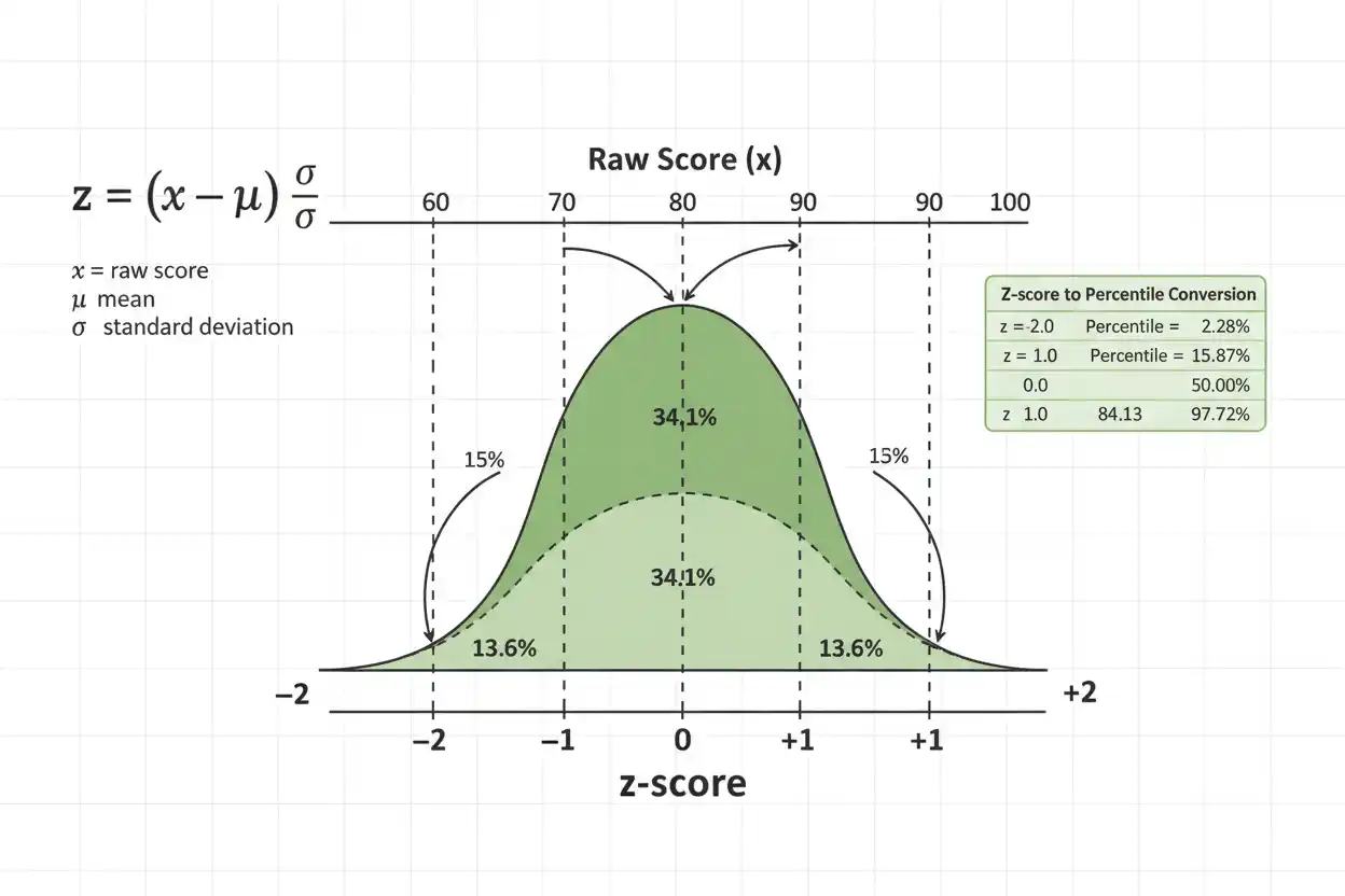
A z-score is a standardized value that measures how far an observation lies from a distribution’s mean in units of standard deviation, allowing values from different scales to be compared on a common numerical basis. A positive z-score indicates that the observation is above the mean, a negative z-score indicates that it is below the mean, and a z-score of zero means that the observation equals the mean exactly. The basic population formula is z = (x − μ)/σ, where x is the observation, μ is the population mean, and σ is the population standard deviation, so a value with z = 2 lies two standard deviations above the mean regardless of whether the original variable is measured in dollars, kilograms, seconds, or examination points. Standardization does not change the relative ordering of observations when σ is positive, but it changes the location and scale so the transformed distribution has mean zero and standard deviation one. Z-scores are used to compare relative positions, identify unusually distant values, convert between raw scores and standardized values, calculate normal-distribution probabilities, and construct test statistics when a standard normal reference distribution is appropriate. Their interpretation nevertheless depends on the underlying distribution because statements such as “z = 2 corresponds to about the 97.7th percentile” require a normal-distribution assumption rather than following from the z-score formula alone.
The z-score is one of the fundamental ideas within core statistics and the broader Statistics & Probability framework. It combines the centering concepts introduced in statistics basics with measures of spread, particularly standard deviation, to express observations on a dimensionless standardized scale.
What Is a Z-Score?
A z-score tells you how many standard deviations an observation is above or below the mean.
The population z-score formula is:
z = (x − μ)/σ
where:
- z = z-score
- x = observed value
- μ = population mean
- σ = population standard deviation
Suppose a population has:
μ = 100
and:
σ = 15
If:
x = 130
then:
z = (130 − 100)/15
z = 30/15
z = 2
Therefore, 130 lies:
2 standard deviations above the population mean.
The z-score has no physical measurement unit because the numerator and denominator are expressed in the same units and therefore cancel.
How to Interpret a Z-Score
The sign tells you the direction relative to the mean.
If:
z > 0
the value is above the mean.
If:
z < 0
the value is below the mean.
If:
z = 0
the value equals the mean.
The magnitude:
|z|
tells you how many standard deviations separate the observation from the mean.
For example:
z = 0.5
means half a standard deviation above the mean.
z = −1.7
means 1.7 standard deviations below the mean.
z = 3
means three standard deviations above the mean.
The numerical distance is standardized, so the same z-score has the same relative meaning across measurement scales, although its probability interpretation can differ when the underlying distributions have different shapes.
Z-Score Formula
The standard population formula is:
z = (x − μ)/σ
The numerator:
x − μ
is the deviation of the observation from the population mean.
Dividing by:
σ
converts that raw deviation into standard-deviation units.
For example, a raw deviation of:
20 points
can be relatively large in a population whose standard deviation is 5, but modest in one whose standard deviation is 50.
A z-score accounts for that difference.
If:
x − μ = 20
and:
σ = 5
then:
z = 4
whereas if:
σ = 50
then:
z = 0.4
The same raw deviation therefore has very different standardized meaning depending on population variability.
Z-Score Example
Suppose examination scores have:
μ = 70
σ = 8
and a student scores:
x = 86
Calculate:
z = (86 − 70)/8
z = 16/8
z = 2
Therefore, the score is:
2 standard deviations above the mean.
Now consider another student with:
x = 62
Then:
z = (62 − 70)/8
z = −8/8
z = −1
The second score is:
1 standard deviation below the mean.
The z-score immediately communicates the positions of both scores relative to the same distribution.
Z-Score of the Mean
The mean itself has:
x = μ
Therefore:
z = (μ − μ)/σ
z = 0
Thus, every distribution with a finite positive standard deviation has its mean at:
z = 0
after standardization.
This remains true even if the distribution is strongly skewed.
Standardizing a skewed distribution centers its mean at zero, but it does not make the distribution symmetric or normal.
Positive Z-Scores
A positive z-score means:
x > μ
Suppose:
μ = 40
σ = 5
and:
x = 47.5
Then:
z = (47.5 − 40)/5
= 7.5/5
= 1.5
The observation lies:
1.5 standard deviations above the mean.
A positive z-score does not necessarily mean the observation is unusually high. A value of:
z = 0.2
is only slightly above the mean.
Whether a positive score is unusual depends on its magnitude and the distributional context.
Negative Z-Scores
A negative z-score means:
x < μ
Suppose:
μ = 50
σ = 10
and:
x = 25
Then:
z = (25 − 50)/10
= −25/10
= −2.5
Therefore, the observation lies:
2.5 standard deviations below the mean.
The negative sign indicates direction only.
A z-score of:
−2.5
and one of:
+2.5
have equal standardized distance from the mean, though they occur on opposite sides.
Z-Score of Zero
If:
z = 0
then:
x = μ
A zero z-score does not mean the original raw value is zero.
For example, if:
μ = 500
then:
x = 500
has:
z = 0
Similarly, if:
μ = −20
then:
x = −20
also has:
z = 0
The standardized zero represents the distribution’s mean, whatever numerical value that mean has on the original measurement scale.
Converting a Z-Score Back to a Raw Score
Start with:
z = (x − μ)/σ
Multiply both sides by σ:
zσ = x − μ
Then add μ:
x = μ + zσ
This is the inverse z-score formula.
If:
μ = 80
σ = 12
and:
z = 1.5
then:
x = 80 + 1.5(12)
x = 80 + 18
x = 98
Therefore, a z-score of 1.5 corresponds to a raw score of:
98
in that distribution.
Raw Score Conversion Example
Suppose a variable has:
μ = 200
σ = 30
What raw value corresponds to:
z = −1.2?
Use:
x = μ + zσ
Then:
x = 200 + (−1.2)(30)
x = 200 − 36
x = 164
Therefore:
z = −1.2
corresponds to:
x = 164.
The value is 36 units below the mean, and 36 equals:
1.2 × 30
standard-deviation units.
Why Z-Scores Are Unitless
The numerator:
x − μ
has the same units as x.
The denominator:
σ
also has the same units.
Therefore:
z = units/units
and the units cancel.
Suppose x is measured in centimeters:
z = centimeters/centimeters
which produces a dimensionless number.
This allows z-scores from variables measured on different scales to be compared meaningfully in terms of standardized position, provided such a comparison makes substantive sense.
Comparing Scores From Different Scales
Suppose Student A scores:
85
on Test A, where:
μA = 70
σA = 10
Then:
zA = (85 − 70)/10
= 1.5
Student B scores:
540
on Test B, where:
μB = 500
σB = 20
Then:
zB = (540 − 500)/20
= 2
Although:
540 > 85
the raw scores are on incomparable scales.
The standardized scores show that Student B is farther above the relevant test mean:
zB = 2
compared with:
zA = 1.5
Thus, Student B has the higher relative standing in standard-deviation units.
Standardization
Converting every observation X into:
Z = (X − μ)/σ
is called standardization.
The transformation does two things.
First, subtracting μ centers the distribution:
X − μ
has mean zero.
Second, dividing by σ rescales its standard deviation to one.
Therefore, when σ > 0:
E(Z) = 0
and:
Var(Z) = 1
so:
SD(Z) = 1
These properties hold whenever the original mean and variance exist and σ is positive.
They do not require normality.
Proving the Standardized Mean Is Zero
Start with:
Z = (X − μ)/σ
Take the expected value:
E(Z) = E[(X − μ)/σ]
Because σ is a constant:
E(Z) = [E(X) − μ]/σ
Since:
E(X) = μ
we obtain:
E(Z) = (μ − μ)/σ
= 0
Therefore, standardization centers the variable at zero.
Proving the Standardized Variance Is One
Again:
Z = (X − μ)/σ
Subtracting a constant does not change variance:
Var(X − μ) = Var(X)
and dividing by σ scales variance by:
1/σ²
Therefore:
Var(Z) = Var(X)/σ²
Since:
Var(X) = σ²
we obtain:
Var(Z) = σ²/σ²
= 1
This relationship follows directly from the transformation rules for variance.
Z-Scores Preserve Ordering
When:
σ > 0
the transformation:
z = (x − μ)/σ
is strictly increasing in x.
Therefore, if:
x₁ < x₂
then:
z₁ < z₂
Standardization does not change which observation is larger.
It changes only the origin and measurement scale.
This means rankings and percentile positions are preserved when values are converted into z-scores using the same mean and positive standard deviation.
Z-Scores Preserve Distribution Shape
Subtracting the mean and dividing by a positive constant are linear transformations.
Therefore, standardization preserves the basic shape of the distribution.
If the original data are:
- right-skewed,
- left-skewed,
- bimodal,
- heavy-tailed,
the standardized data retain those structural characteristics.
The mean becomes zero and standard deviation becomes one, but the distribution does not automatically become bell-shaped.
This distinction is essential because the term “standard score” is sometimes incorrectly treated as synonymous with “normally distributed score.”
Z-Score and the Standard Normal Distribution
If the original variable is normally distributed:
X ~ N(μ, σ²)
then standardizing gives:
Z = (X − μ)/σ
and:
Z ~ N(0,1)
This is the standard normal distribution.
Its mean is:
0
and variance:
1
Because every normal distribution can be transformed into the same standard normal distribution, probabilities for any normal model can be calculated using standard normal probabilities after conversion to z.
This is one of the most important uses of z-scores.
Normal Probability Example
Suppose:
X ~ N(100, 15²)
Find:
P(X ≤ 130)
First standardize:
z = (130 − 100)/15
z = 2
Therefore:
P(X ≤ 130) = P(Z ≤ 2)
For the standard normal distribution:
P(Z ≤ 2) ≈ 0.97725
Thus:
P(X ≤ 130) ≈ 97.73%
and:
P(X > 130) ≈ 2.28%
The probability calculation requires the normal-distribution assumption.
The z-score value of 2 by itself does not guarantee those percentages for an arbitrary distribution.
Z-Score and Percentile
Under a standard normal model, a z-score maps directly to a cumulative percentile through the standard normal CDF:
Percentile probability = Φ(z)
where Φ is the cumulative distribution function of:
N(0,1)
For example:
z = 0 → 50th percentile
approximately:
z = 1 → 84.13th percentile
z = 1.645 → 95th percentile
z = 1.96 → 97.5th percentile
z = 2.326 → 99th percentile
Similarly:
z = −1.645
corresponds approximately to the 5th percentile.
These conversions are normal-specific.
Finding a Raw Score From a Normal Percentile
Suppose:
X ~ N(500, 100²)
and we want the 90th percentile.
The standard-normal 90th-percentile value is approximately:
z₀.₉₀ = 1.2816
Use:
x = μ + zσ
Then:
x = 500 + 1.2816(100)
x = 500 + 128.16
x ≈ 628.16
Therefore, the 90th percentile is approximately:
628.2
under this normal model.
Z-Score and the Empirical Rule
For a normal distribution, approximately:
68.27%
of observations fall between:
z = −1 and z = 1
approximately:
95.45%
fall between:
z = −2 and z = 2
and approximately:
99.73%
fall between:
z = −3 and z = 3
This is the familiar 68–95–99.7 rule.
It provides an intuitive interpretation of z-score magnitude when normality is reasonable.
It should not be applied automatically to strongly non-normal distributions.
Is a Z-Score Above 2 an Outlier?
A z-score with magnitude above 2 is sometimes described informally as unusual, but:
|z| > 2
is not a universal definition of an outlier.
Under a normal distribution, about:
4.55%
of observations lie outside ±2 standard deviations.
That is uncommon but not extraordinarily rare.
Likewise:
|z| > 3
corresponds to a much more extreme normal-tail position, yet even that does not prove an observation is erroneous.
Outlier assessment should incorporate distribution shape, sample size, measurement quality, and context rather than rely on a rigid z cutoff alone.
Z-Score Outlier Example
Suppose:
μ = 50
σ = 5
and an observation is:
x = 70
Then:
z = (70 − 50)/5
= 4
Under an exact normal model, z = 4 is an extremely high-tail observation.
However, several interpretations remain possible:
- a valid rare observation,
- a recording error,
- a population subgroup,
- a change in the underlying process,
- a non-normal distribution.
The z-score identifies standardized extremeness relative to the chosen mean and standard deviation. It does not identify the cause.
Sample Z-Score
When only sample statistics are available, observations are often standardized descriptively using:
zᵢ = (xᵢ − x̄)/s
where:
- x̄ = sample mean
- s = sample standard deviation
This is frequently called a sample z-score or standardized sample score.
It is useful for describing where observations lie relative to their own sample.
However, it is conceptually different from the population standardization:
(x − μ)/σ
because both the center and scale are estimated from the same sample.
The resulting standardized sample values have special finite-sample identities.
Mean of Sample Z-Scores
If:
zᵢ = (xᵢ − x̄)/s
then:
Σzᵢ = (1/s)Σ(xᵢ − x̄)
Because:
Σ(xᵢ − x̄) = 0
we obtain:
Σzᵢ = 0
Therefore, the arithmetic mean of the standardized sample values is:
0
provided s > 0.
This is an exact property of sample standardization.
Sample Standard Deviation of Sample Z-Scores
Using:
zᵢ = (xᵢ − x̄)/s
where s is the conventional sample standard deviation:
s² = Σ(xᵢ − x̄)²/(n − 1)
we have:
Σzᵢ²
= Σ(xᵢ − x̄)²/s²
Since:
Σ(xᵢ − x̄)² = (n − 1)s²
it follows that:
Σzᵢ² = n − 1
Therefore, the sample variance of the zᵢ values is:
1
and their sample standard deviation is:
1
when calculated with the same n − 1 convention.
Sample Z-Score Example
Consider the sample:
10, 12, 14, 16, 18
The sample mean is:
x̄ = 14
The squared deviations are:
16, 4, 0, 4, 16
so:
s² = 40/(5 − 1)
s² = 10
and:
s ≈ 3.1623
For:
x = 18
the sample-standardized score is:
z = (18 − 14)/3.1623
z ≈ 1.2649
For:
x = 10
we obtain:
z ≈ −1.2649
The scores are symmetric because the original sample is symmetric around 14.
Population vs Sample Z-Score
The population z-score uses:
z = (x − μ)/σ
The descriptive sample-standardized score uses:
z = (x − x̄)/s
These formulas resemble one another but do not have identical probabilistic meaning.
The population formula standardizes relative to fixed population parameters.
The sample formula standardizes relative to statistics estimated from the same observed sample.
A sample-standardized score should not automatically be interpreted using exact standard-normal probabilities merely because it has been labeled a z-score.
Normal-tail probability interpretation requires an appropriate probabilistic model.
Z-Score vs Z-Test Statistic
A raw-observation z-score and a z-test statistic share the idea of standardization, but their denominators represent different kinds of variation.
For an individual observation:
z = (x − μ)/σ
For a sample mean under a known-σ null hypothesis:
z = (x̄ − μ₀)/(σ/√n)
The individual z-score divides by the standard deviation of observations.
The z-test statistic divides by the standard deviation of the sampling distribution of the mean, which is:
σ/√n
Therefore, a modest difference in raw units can produce a large test statistic when n is large because sample means are much less variable than individual observations.
Individual Z-Score vs Z-Test Example
Suppose:
μ = 100
σ = 20
An individual value:
x = 104
has:
z = (104 − 100)/20
= 0.2
so it is only 0.2 standard deviations above the mean.
Now suppose a sample of:
n = 100
has:
x̄ = 104
The sampling standard deviation of the mean is:
20/√100
= 2
Therefore, the mean-based z statistic is:
z = (104 − 100)/2
= 2
The same raw difference of four units is much more unusual for an average of 100 independent observations than for one individual observation.
Z-Score vs t Statistic
A t-test also standardizes an estimated difference, but it generally uses an estimated population standard deviation.
For a one-sample mean:
t = (x̄ − μ₀)/(s/√n)
By contrast, a classical known-σ mean z statistic uses:
z = (x̄ − μ₀)/(σ/√n)
The formulas differ in whether the relevant population standard deviation is known or estimated.
Because estimating σ introduces additional uncertainty, the t statistic is compared with a Student’s t distribution rather than an exact standard normal distribution under the classical small-sample normal model.
As degrees of freedom increase, t and z reference distributions become increasingly similar.
Z-Score and Variance
Because:
σ = √σ²
the z-score can also be expressed using variance:
z = (x − μ)/√σ²
The denominator therefore represents the square root of population variance.
Variance itself is measured in squared units, so using σ rather than σ² in the z-score returns the denominator to the original units of x.
This makes:
x − μ
and:
σ
directly comparable before their units cancel.
Effect of Changing Units
Suppose temperature-like measurements are transformed using:
Y = aX + b
with:
a > 0
The z-score is unchanged when the mean and standard deviation are transformed consistently.
Since:
μY = aμX + b
and:
σY = aσX
we have:
zY = [aX + b − (aμX + b)]/(aσX)
= a(X − μX)/(aσX)
= zX
Therefore, positive linear unit conversions preserve z-scores.
This is why standardized position is independent of whether a quantity is expressed, for example, in meters or centimeters.
Negative Linear Transformations
If:
Y = aX + b
with:
a < 0
the ordering reverses.
The standard deviation becomes:
σY = |a|σX
so:
zY = a(X − μX)/(|a|σX)
Therefore:
zY = −zX
when a is negative.
The standardized magnitude remains the same but the sign reverses because values that were above the mean become below the mean after the scale is reversed.
Z-Scores and Percentile Ranks Are Not the Same Thing
A z-score measures standardized distance from the mean.
A percentile rank measures cumulative position within a distribution.
The two are directly connected only after a distributional model is specified.
For a normal distribution:
z = 1
corresponds approximately to the:
84.13th percentile.
For a strongly skewed distribution, an observation one standard deviation above the mean can correspond to a very different percentile.
Thus:
standardized distance
and:
cumulative rank
are distinct statistical concepts.
Z-Scores in Skewed Distributions
Z-scores remain mathematically valid for skewed data when the mean and standard deviation exist.
Suppose a highly right-skewed distribution has:
μ = 100
σ = 80
An observation:
x = 180
has:
z = 1
regardless of the distribution shape.
However, we cannot infer:
“x is at the 84th percentile”
unless the distribution is normal or another known model supplies that percentile relationship.
In a right-skewed distribution, the proportion of observations above or below z = 1 can differ substantially from normal probabilities.
Z-Scores in Heavy-Tailed Distributions
Heavy-tailed distributions contain more extreme observations than a normal distribution with the same mean and variance.
As a result, values such as:
|z| > 3
may occur much more frequently than normal theory predicts.
Using normal-table probabilities mechanically can therefore exaggerate the unusualness of observations from a heavy-tailed population.
A z-score still describes standardized distance, but probability interpretation should come from the actual or assumed distribution.
When theoretical variance is infinite or undefined, population z-standardization itself may not be available in the usual form.
Z-Scores and Outlier Detection
Z-scores are often used as one component of outlier screening because they place observations on a common deviation scale.
Rules such as:
|z| > 2
or:
|z| > 3
are sometimes used as informal screening thresholds.
These are not universal definitions.
Their usefulness depends on:
- distribution shape,
- sample size,
- whether μ and σ are known or estimated,
- whether one or many observations are being screened,
- the cost of false flags.
In small samples, an extreme observation can also inflate x̄ and s, making its own sample z-score less extreme than expected.
Masking in Sample Z-Scores
Suppose one very large observation appears in a small sample.
That observation raises:
x̄
and can substantially increase:
s
because its squared deviation contributes heavily to the variance.
Both changes can reduce the resulting standardized distance:
(x − x̄)/s
for the extreme value.
This phenomenon can contribute to masking, where extreme observations make one another or themselves appear less unusual under mean-and-standard-deviation-based diagnostics.
Robust approaches using medians and resistant scale estimates may therefore complement z-score screening when contamination is a concern.
Z-Scores and Data Comparison
Z-scores can be useful when comparing measurements that have different means and spreads.
Suppose:
Variable A: x = 120, μ = 100, σ = 10
Then:
zA = 2
Suppose:
Variable B: x = 80, μ = 50, σ = 20
Then:
zB = 1.5
Even though the raw deviations are:
20 for A
and:
30 for B
A is more extreme relative to its own distribution because its deviation equals two standard deviations rather than 1.5.
The standardized comparison accounts for scale-specific variability.
Z-Scores Do Not Make Variables Equally Important
Standardizing several variables gives each a mean near zero and standard deviation near one under the chosen sample or population definitions, but this does not make the variables equally useful, reliable, or substantively important.
A noisy variable and a highly informative variable can both be standardized to unit variance.
Standardization changes scale.
It does not improve measurement quality, eliminate confounding, make distributions normal, or determine causal relevance.
This distinction is especially important when standardized variables enter multivariable models.
Z-Scores in Regression
Predictors are sometimes standardized before regression:
Zx = (X − μX)/σX
or, in sample work:
zx = (x − x̄)/sX
A regression coefficient for a standardized predictor can then describe the fitted response change associated with a one-standard-deviation increase in that predictor.
If the response is also standardized, the coefficient becomes dimensionless in simple linear regression and relates closely to correlation.
However, standardization does not change the underlying explanatory quality of the data. It changes the coefficient scale and can improve interpretability or numerical comparability in selected settings.
Z-Scores and Correlation
If both X and Y are standardized using population quantities:
ZX = (X − μX)/σX
ZY = (Y − μY)/σY
then their covariance is:
Cov(ZX, ZY)
which equals the correlation:
ρXY
because both standardized variables have standard deviation one.
Thus:
Corr(X,Y) = E(ZXZY)
under the population formulation.
This relationship shows how correlation can be understood as the expected product of standardized deviations.
A positive product occurs when both variables tend to lie on the same side of their respective means.
Z-Scores and Covariance
The population covariance is:
Cov(X,Y) = E[(X − μX)(Y − μY)]
Divide by both standard deviations:
Cov(X,Y)/(σXσY)
to obtain correlation.
Because:
ZX = (X − μX)/σX
and:
ZY = (Y − μY)/σY
we can write:
ρ = E(ZXZY)
This is another reason standardization is useful: it removes measurement units from joint variation.
Covariance retains units; correlation and z-scores do not.
Z-Scores and the Sample Mean
A raw-score z transformation and a sample-mean test statistic should not be confused.
For one observation:
z = (x − μ)/σ
For a sample mean:
z_mean = (x̄ − μ)/(σ/√n)
The second denominator is much smaller when n is large.
For example, if:
σ = 20
and:
n = 100
then:
σ/√n = 2
Therefore, a sample mean only four units from μ is:
2 standard errors
away even though an individual observation four units from μ is only:
0.2 standard deviations
away.
Z-Scores and Standard Error
A standard deviation describes the spread of individual values.
A standard error describes the spread of an estimator across repeated samples.
A z-score can be built using either scale depending on what is being standardized.
For an individual:
Standardized observation = deviation / observation SD
For an estimator:
Standardized statistic = estimation error / standard error
The second form is used in many inferential procedures.
Understanding which denominator appears in a formula is essential because the two z-values can differ dramatically.
Finding an Unknown Mean From a Z-Score
Start with:
z = (x − μ)/σ
Multiply by σ:
zσ = x − μ
Rearrange:
μ = x − zσ
Suppose:
x = 75
z = 1.5
σ = 10
Then:
μ = 75 − 1.5(10)
μ = 75 − 15
μ = 60
Therefore, a value of 75 has z = 1.5 when the mean is 60 and standard deviation is 10.
Finding an Unknown Standard Deviation
Starting from:
z = (x − μ)/σ
solve for σ:
σ = (x − μ)/z
provided:
z ≠ 0
Suppose:
x = 90
μ = 70
z = 2.5
Then:
σ = (90 − 70)/2.5
= 20/2.5
= 8
Therefore:
σ = 8
The signs must be consistent: x − μ and z have the same sign because σ is positive.
Z-Score With Decimal Values
Z-scores do not need to be integers.
Suppose:
x = 53.7
μ = 48.2
σ = 4.4
Then:
z = (53.7 − 48.2)/4.4
= 5.5/4.4
= 1.25
The observation is:
1.25 standard deviations above the mean.
Decimal z-scores are ordinary and often provide more precise standardized positions than rounding to whole standard deviations.
Z-Score With Negative Raw Values
Raw observations can be negative without causing any problem.
Suppose:
μ = −10
σ = 4
and:
x = −2
Then:
z = [−2 − (−10)]/4
= 8/4
= 2
Although x itself is negative, it lies two standard deviations above the mean because −2 is greater than −10.
The z-score sign depends on position relative to the mean, not whether the raw number is positive or negative.
Z-Score When Standard Deviation Is Zero
If:
σ = 0
then every population observation equals the same value μ.
The formula:
z = (x − μ)/σ
would require division by zero.
Therefore, ordinary z-scores are undefined when standard deviation is zero.
Conceptually, there is no dispersion scale available for standardization.
If all observations are identical, relative distance in standard-deviation units is not meaningful.
Rounding Z-Scores
Intermediate calculations should generally preserve enough decimal precision to avoid materially changing the final result.
For example:
z = 1.9647
might be reported as:
z ≈ 1.96
for ordinary interpretation.
However, rounding too early can noticeably alter tail probabilities, especially in extreme regions where small changes in z correspond to meaningful relative changes in very small probabilities.
A good practice is to calculate with full available precision and round only the reported final value.
Common Z-Score Values Under Normality
Under a standard normal distribution, several z-scores appear frequently:
| z-score | Approximate cumulative probability |
|---|---|
| −2.326 | 0.01 |
| −1.960 | 0.025 |
| −1.645 | 0.05 |
| 0 | 0.50 |
| 1.645 | 0.95 |
| 1.960 | 0.975 |
| 2.326 | 0.99 |
These values are especially important for confidence intervals and hypothesis testing.
They are standard-normal quantiles, not universal percentile relationships for every standardized distribution.
Why 1.96 Appears So Often
For a standard normal variable Z:
P(−1.96 ≤ Z ≤ 1.96) ≈ 0.95
More precisely, approximately 2.5% lies below:
−1.96
and approximately 2.5% lies above:
1.96.
Therefore, ±1.96 defines the central 95% of the standard normal distribution.
This is why:
1.96
appears in many large-sample 95% confidence procedures.
The value comes from the standard normal probability distribution rather than from an arbitrary statistical convention.
Z-Score and Confidence Intervals
A large-sample confidence interval often has the structure:
Estimate ± z* × Standard error
where z* is a standard-normal critical value.
For a 95% procedure:
z* ≈ 1.96
Suppose:
Estimate = 50
and:
SE = 3
Then:
Margin = 1.96(3)
= 5.88
so the interval is:
50 ± 5.88
or:
(44.12, 55.88)
Here the critical z-score identifies the standardized distance needed to capture the desired central probability under the reference distribution.
Z-Scores and Hypothesis Testing
A hypothesis-test statistic often has the same standardized structure:
z = (Estimate − Null value)/SE
Suppose:
Estimate = 105
Null value = 100
SE = 2
Then:
z = (105 − 100)/2
= 2.5
Under a standard-normal null reference distribution, a two-sided result of:
|z| = 2.5
corresponds to a relatively small p-value.
This inferential use of z should be distinguished from the descriptive z-score of an individual observation, even though the standardization principle is the same.
Z-Score vs T-Score
In statistical inference, a t statistic differs from a z statistic mainly because the relevant variance is estimated and the resulting reference distribution has heavier tails.
However, the term T-score can also refer in some testing contexts to a transformed score with a chosen mean and standard deviation, such as:
T = 50 + 10z
That transformed-score usage is different from Student’s t statistic.
The meaning must therefore be determined from context.
A standard z-score conventionally has:
mean 0
and:
standard deviation 1
while other standardized scoring systems can intentionally use different centers and scales.
Alternative Standard Score Scales
A z-score can be linearly transformed into another standardized scale.
Suppose:
T = 50 + 10z
Then:
z = 0 → T = 50
z = 1 → T = 60
z = −1 → T = 40
The ordering and relative standardized position remain unchanged.
Similarly, a scoring system can choose another mean and standard deviation for convenience.
These transformations can make scores easier to communicate while preserving the same underlying standardized ranking.
Common Z-Score Mistakes
A common mistake is reversing the numerator and calculating:
(μ − x)/σ
instead of:
(x − μ)/σ.
That reverses every sign and therefore reverses whether observations are interpreted as above or below the mean.
Another error is dividing by variance:
σ²
rather than standard deviation:
σ.
The z-score denominator must have the same units as the numerator.
Another common mistake is interpreting every z-score through a normal-distribution table even when the underlying distribution is strongly skewed or otherwise non-normal. Standardization alone does not create normality.
Analysts also frequently confuse an individual z-score with a z-test statistic for a sample mean. The former uses σ; the latter can use:
σ/√n
because it standardizes a sample estimator rather than an individual observation.
Another mistake is assuming:
|z| > 2
automatically proves an observation is an outlier or error.
It is also incorrect to calculate a z-score when the relevant standard deviation is zero.
Finally, using x̄ and s in place of μ and σ changes the calculation into sample-based standardization and should be interpreted accordingly.
How to Calculate a Z-Score Step by Step
Begin by identifying the observation x, the appropriate mean, and the appropriate standard deviation. Determine whether you are standardizing relative to known population parameters:
μ and σ
or descriptively relative to sample statistics:
x̄ and s.
For population standardization, calculate the raw deviation:
x − μ
Then divide by the population standard deviation:
z = (x − μ)/σ
Check the sign: values above the mean should have positive z-scores, while values below the mean should have negative z-scores.
Finally, interpret the magnitude as a distance in standard-deviation units. Convert the z-score into a percentile or tail probability only when a probability distribution—commonly the normal distribution—has been specified.
Full Z-Score Worked Example
Suppose a population of measurements has:
μ = 72
σ = 6
and an observation is:
x = 84
Step 1: Find the Deviation
x − μ = 84 − 72
= 12
Step 2: Divide by Standard Deviation
z = 12/6
= 2
Step 3: Interpret
The observation lies:
2 standard deviations above the population mean.
If the population is normally distributed:
P(Z ≤ 2) ≈ 0.97725
so the observation is approximately at the:
97.7th percentile.
The upper-tail probability is approximately:
1 − 0.97725
= 0.02275
or:
2.28%
Again, the percentile and tail statements depend on normality; the standardized distance does not.
Full Negative Z-Score Example
Suppose:
μ = 500
σ = 40
and:
x = 420
Then:
z = (420 − 500)/40
= −80/40
= −2
The observation lies:
2 standard deviations below the mean.
If X is normally distributed, its cumulative probability is approximately:
P(Z ≤ −2) ≈ 0.02275
so roughly:
2.28%
of the normal distribution lies below this value.
Its relative location is therefore symmetric with a z-score of +2 on the opposite side of the mean.
Full Comparison Example
Suppose a person has:
Score A = 88
where:
μA = 76
σA = 8
and:
Score B = 640
where:
μB = 580
σB = 50
For Score A:
zA = (88 − 76)/8
= 12/8
= 1.5
For Score B:
zB = (640 − 580)/50
= 60/50
= 1.2
Although Score B has the larger raw numerical value and larger raw deviation from its mean, Score A has the stronger relative standing:
1.5 standard deviations above its mean
compared with:
1.2 standard deviations above the mean.
This is precisely the kind of comparison z-scores are designed to facilitate.
How to Report a Z-Score
A clear z-score statement should include both the standardized value and its interpretation in original context.
For example:
“The observation was 84 in a population with mean 72 and standard deviation 6, corresponding to z = 2.00, or two standard deviations above the mean.”
If normality is justified and a percentile is relevant, it can be added separately:
“Under a normal-distribution model, z = 2 corresponds to approximately the 97.7th percentile.”
Keeping the standardized-distance statement separate from the distribution-dependent probability statement prevents the normality assumption from being hidden.
When sample mean and sample standard deviation are used instead of population parameters, identify the score as standardized relative to the observed sample.
Frequently Asked Questions About the Z-Score
What is a z-score?
A z-score measures how far a value lies above or below a mean in standard-deviation units.
What is the z-score formula?
For population standardization:
z = (x − μ)/σ
What does a positive z-score mean?
The observation lies above the mean.
What does a negative z-score mean?
The observation lies below the mean.
What does z = 0 mean?
The observation equals the mean.
What does z = 1 mean?
The observation lies one standard deviation above the mean.
What does z = −2 mean?
The observation lies two standard deviations below the mean.
Can a z-score be greater than 3?
Yes. Z-scores are not restricted to the interval −3 to 3.
Can a z-score be negative?
Yes.
Can a raw negative value have a positive z-score?
Yes. If the raw value is greater than the mean, its z-score is positive even when both numbers are negative.
Does a z-score have units?
No. It is dimensionless because the measurement units cancel.
How do you convert a z-score into a raw score?
Use:
x = μ + zσ
How do you find the mean from a z-score?
Use:
μ = x − zσ
How do you find standard deviation from a z-score?
When z ≠ 0:
σ = (x − μ)/z
What is standardization?
Standardization transforms:
X
into:
Z = (X − μ)/σ
so the transformed variable has mean zero and variance one when μ and σ are the true population parameters.
Does standardization make data normal?
No. It changes location and scale but preserves the distribution’s basic shape.
What is the mean of standardized population scores?
0
What is their standard deviation?
1
provided the original population standard deviation is positive and finite.
What is a sample z-score?
A common descriptive sample-standardization formula is:
zᵢ = (xᵢ − x̄)/s
Are sample z-scores exactly standard normal?
No. Having sample mean zero and sample standard deviation one does not make their distribution normal.
Is a z-score the same as a percentile?
No. A z-score measures standardized distance, while a percentile measures cumulative rank.
How are z-scores converted to percentiles?
A distribution must be specified. Under a normal model:
Percentile probability = Φ(z)
What percentile is z = 0 in a normal distribution?
50th percentile
What percentile is z = 1?
Approximately:
84.13th percentile
under a normal distribution.
What percentile is z = 1.645?
Approximately:
95th percentile
under a standard normal distribution.
What percentile is z = 1.96?
Approximately:
97.5th percentile
for cumulative probability, while ±1.96 encloses approximately the central 95% of a standard normal distribution.
What percentile is z = 2.326?
Approximately:
99th percentile
under the standard normal model.
Is z = 2 always the 97.7th percentile?
No. That relationship is specific to a normal distribution.
Is a z-score above 2 an outlier?
Not automatically. It may be unusual under some distributions, but outlier classification requires additional statistical and contextual judgment.
Is z = 3 an error?
No. A value three standard deviations from the mean can be a legitimate observation.
Why do z-scores use standard deviation rather than variance?
Standard deviation has the same units as x − μ, so the units cancel and the resulting score is dimensionless.
What is the relationship between variance and a z-score?
Since:
σ = √σ²
the formula can be written:
z = (x − μ)/√σ²
What is the difference between a z-score and a z-test statistic?
An individual z-score usually standardizes one observation using σ, while a z-test statistic standardizes an estimator using its standard error, such as σ/√n for a sample mean.
What is the difference between z and t?
A classical z statistic uses a known or specified population standard deviation or asymptotic standard error. A t statistic typically uses an estimated standard deviation and a Student’s t reference distribution.
Does sample size affect an individual z-score?
Not directly when μ and σ are fixed population parameters.
Does sample size affect a z-test statistic for a sample mean?
Yes. Its standard error is:
σ/√n
so larger n makes the sampling distribution of the mean narrower.
Can two different raw scores have the same z-score?
Yes, if they come from different distributions and occupy the same standardized position relative to their respective means and standard deviations.
Can two observations in the same distribution have the same z-score?
Only if they have the same raw value when μ and σ are fixed and σ > 0.
Does changing measurement units change the z-score?
A positive linear unit conversion does not change the z-score when the mean and standard deviation are converted consistently.
What happens if all observations are identical?
Then:
σ = 0
and ordinary z-scores are undefined because there is no nonzero dispersion scale.
What is the main advantage of a z-score?
It converts raw deviations into a common standard-deviation scale, making relative positions easier to interpret and compare across distributions.
What is the most important rule when interpreting a z-score?
Interpret the sign and magnitude as standardized distance first, and use normal percentiles or tail probabilities only when a normal-distribution assumption is justified.




