Five-Number Summary: Definition, Formula & Example

Mehran Khan Last Updated: August 31, 2026

0 2 23 minutes read

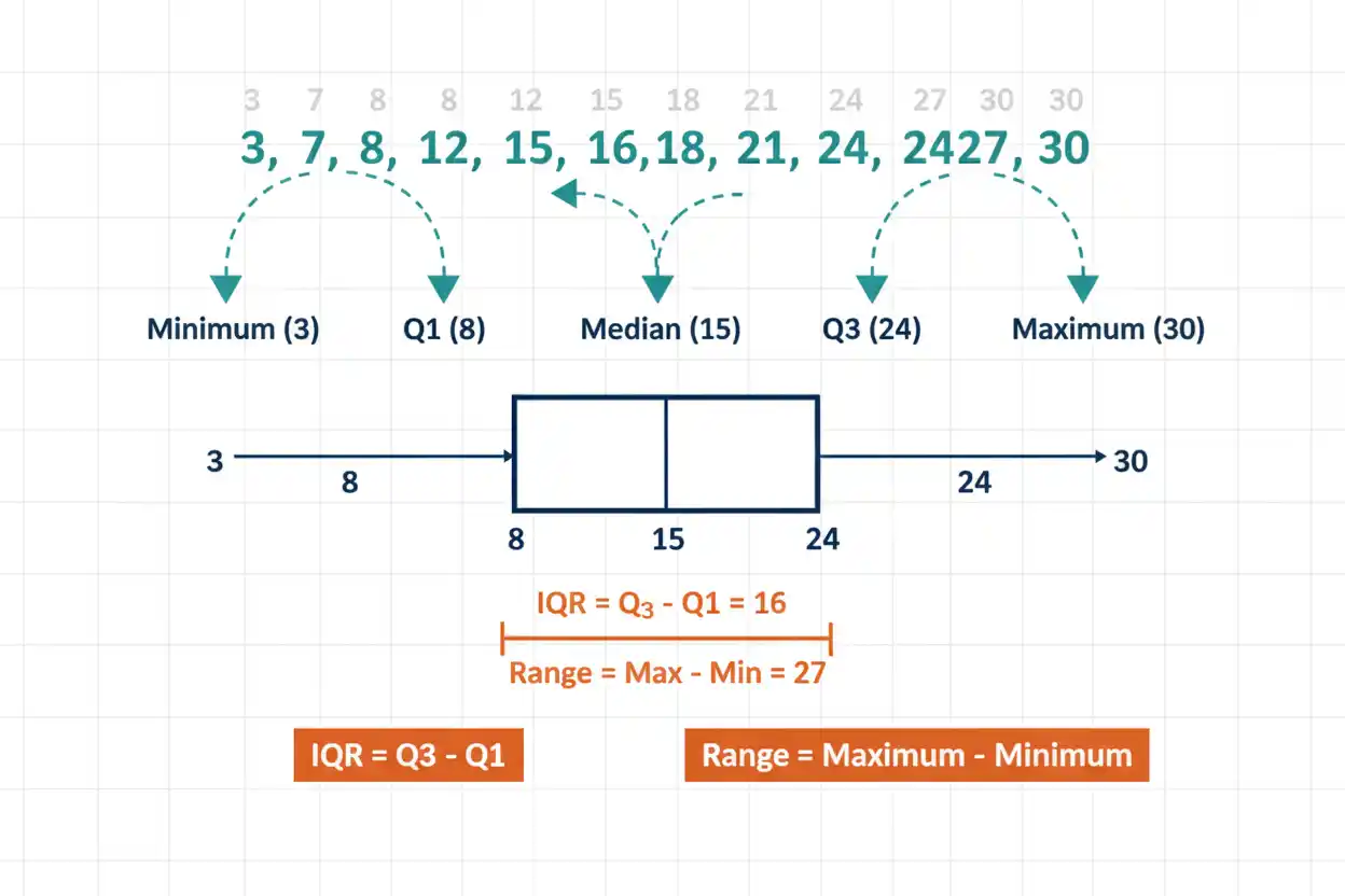
A five-number summary is a compact description of a numerical distribution using its minimum, first quartile Q₁, median Q₂, third quartile Q₃, and maximum, allowing the location, central spread, overall range, and possible asymmetry of a data set to be understood without displaying every observation. These five positional statistics divide an ordered distribution into meaningful regions: the minimum and maximum define the observed endpoints, the median identifies the central ranked value, and Q₁ and Q₃ mark the lower and upper boundaries of the middle half of the data. From the same quantities, the interquartile range can be calculated as IQR = Q₃ − Q₁ and the ordinary range as maximum − minimum, providing two complementary measures of spread. Because the summary is based primarily on ranks rather than squared deviations from an arithmetic center, its central components are relatively resistant to a small number of extreme observations, making it especially useful for skewed or heavy-tailed data. The exact numerical values of Q₁ and Q₃ can nevertheless differ among accepted quartile conventions, particularly in small samples, so the calculation method should be identified whenever exact reproducibility matters.

The five-number summary is a fundamental tool within descriptive statistics and the broader Statistics & Probability framework. It also provides the numerical foundation for quartile-based visualizations because the same ordered landmarks describe how observations are positioned from the lower end of a distribution through its center to its upper end.

What Is a Five-Number Summary?

A five-number summary consists of:

Minimum

First quartile: Q₁

Median: Q₂

Third quartile: Q₃

Maximum

It is commonly written as the ordered tuple:

(Minimum, Q₁, Median, Q₃, Maximum)

Suppose a data set has:

Minimum = 2

Q₁ = 5

Median = 9

Q₃ = 13

Maximum = 18

Then its five-number summary is:

(2, 5, 9, 13, 18)

These values describe the principal ranked locations of the distribution without requiring a reader to examine every observation individually.

What Each Number Means

The five quantities represent different positions in the ordered data.

The minimum is the smallest observed value.

Q₁ corresponds conceptually to the 25th-percentile region.

The median corresponds to the 50th percentile.

Q₃ corresponds conceptually to the 75th-percentile region.

The maximum is the largest observed value.

Together they divide the distribution into four broad ranked sections containing approximately equal fractions of the observations, although exact finite-sample definitions depend on the quartile convention.

Five-Number Summary Formula

There is no single arithmetic formula that simultaneously generates all five quantities, because the summary combines endpoints and ordered quantiles.

Its structure can be written:

Five-number summary = (Min, Q₁, Q₂, Q₃, Max)

with:

Q₂ = Median

Two useful derived formulas are:

IQR = Q₃ − Q₁

and:

Range = Maximum − Minimum

The IQR measures the width of the middle half of the distribution.

The range measures the full observed span.

These two measures behave differently when extreme observations are present.

Step 1: Sort the Data

The observations must be arranged from smallest to largest before quartiles or the median can be found.

Suppose the unsorted data are:

12, 5, 18, 7, 2, 13, 9, 10, 4, 15, 8

Sort them:

2, 4, 5, 7, 8, 9, 10, 12, 13, 15, 18

Now the endpoints and ranked center can be identified correctly.

Attempting to calculate quartiles from the unsorted sequence can produce meaningless positional results.

Ordering is therefore the essential first step.

Step 2: Find the Minimum

The minimum is the first observation after sorting.

For:

2, 4, 5, 7, 8, 9, 10, 12, 13, 15, 18

we have:

Minimum = 2

The minimum represents the lower observed endpoint.

It is not necessarily a lower population boundary.

A future or unobserved value could be smaller if the data are only a sample.

Step 3: Find the Maximum

The maximum is the last observation in the ordered set.

For the same data:

Maximum = 18

The maximum therefore represents the upper observed endpoint.

Like the minimum, it can be highly sensitive to sample size and extreme observations because only one observation determines it.

The minimum and maximum together give the ordinary observed range.

Step 4: Find the Median

The median divides the ordered data into lower and upper halves.

For an odd number n of observations, its position is:

Median position = (n + 1)/2

Here:

n = 11

so:

Median position = (11 + 1)/2

= 6

The sixth observation is:

9

Therefore:

Median = 9

This is also:

Q₂ = 9.

Step 5: Find Q₁

Using the common median-of-halves convention that excludes the overall median when n is odd, the lower half is:

2, 4, 5, 7, 8

The median of these five values is:

5

Therefore:

Q₁ = 5

This value identifies the central position of the lower half under this quartile convention.

Approximately one quarter of the observations lie at or below this region of the ordered distribution.

Step 6: Find Q₃

The upper half is:

10, 12, 13, 15, 18

Its median is:

13

Therefore:

Q₃ = 13

The five-number summary is now complete:

(2, 5, 9, 13, 18)

From it, several additional measures can be calculated immediately.

Full Five-Number Summary Example

For:

2, 4, 5, 7, 8, 9, 10, 12, 13, 15, 18

we found:

Minimum = 2

Q₁ = 5

Median = 9

Q₃ = 13

Maximum = 18

Therefore:

Five-number summary = (2, 5, 9, 13, 18)

This summary shows that the central half of observations lies between:

5 and 13

while the complete observed data span:

2 through 18.

Interquartile Range From the Five-Number Summary

The interquartile range is:

IQR = Q₃ − Q₁

Using:

Q₁ = 5

Q₃ = 13

we obtain:

IQR = 13 − 5

= 8

Therefore, the middle 50% of the ordered data spans:

8 units.

IQR is a resistant measure of central spread because isolated changes to the minimum or maximum usually do not affect it unless those changes alter the quartile positions.

Range From the Five-Number Summary

The ordinary range is:

Range = Maximum − Minimum

Using:

Maximum = 18

and:

Minimum = 2

we obtain:

Range = 18 − 2

= 16

The entire observed sample therefore spans:

16 units.

Unlike IQR, the range depends completely on the two extreme observations.

One unusually large or small value can therefore alter it substantially.

Range vs IQR

Range and IQR describe different portions of the distribution.

The range:

Maximum − Minimum

describes the full observed span.

The IQR:

Q₃ − Q₁

describes the central half.

Suppose an extreme maximum changes from:

18

to:

The range increases dramatically.

However, Q₁ and Q₃ may remain unchanged if the ranked central positions do not move.

The IQR can therefore provide a more stable description of typical spread when tail values are extreme.

Five-Number Summary and Quartiles

Quartiles are the central components of the five-number summary.

They divide the distribution approximately into:

lower quarter

second quarter

third quarter

upper quarter.

The intervals are:

Minimum to Q₁

Q₁ to Median

Median to Q₃

Q₃ to Maximum

Each section contains approximately one quarter of the data by rank, but their numerical widths can differ greatly.

Equal proportions do not imply equal distances on the measurement scale.

Unequal Quartile Widths

Suppose a five-number summary is:

(2, 5, 7, 20, 100)

The four intervals have widths:

5 − 2 = 3

7 − 5 = 2

20 − 7 = 13

100 − 20 = 80

Each represents roughly a quarter of the ranked distribution, yet the upper quarter spans dramatically more numerical space.

This suggests substantial upper-tail dispersion.

The summary therefore provides information about distribution shape in addition to center.

Five-Number Summary and Symmetry

A roughly symmetric summary might look like:

(0, 10, 20, 30, 40)

The distances from the median are balanced:

20 − 10 = 10

30 − 20 = 10

and the outer ranges are also balanced:

10 − 0 = 10

40 − 30 = 10.

This pattern is compatible with a symmetric distribution.

However, it does not prove the distribution is normal or even perfectly symmetric because the five-number summary omits most individual observations.

Five-Number Summary and Right Skew

Consider:

(2, 5, 8, 15, 60)

The upper half is much more spread out than the lower half.

From median to Q₃:

15 − 8 = 7

while from Q₁ to median:

8 − 5 = 3.

The upper tail:

60 − 15 = 45

is also much longer than the lower tail:

5 − 2 = 3.

These features are consistent with a right-skewed distribution.

They provide a descriptive indication, not a formal proof of skewness.

Five-Number Summary and Left Skew

A pattern such as:

(−40, 5, 12, 15, 18)

has a much longer lower tail.

The distance from minimum to Q₁ is:

5 − (−40)

= 45

while the distance from Q₃ to maximum is:

18 − 15

= 3.

This arrangement is consistent with left skew.

Again, a histogram or other full-distribution graphic can reveal shape more completely because five values cannot preserve every feature.

Median With an Even Number of Observations

Suppose the ordered data are:

2, 4, 6, 8, 10, 12, 14, 16

Here:

n = 8

The middle positions are:

4th and 5th.

The observations are:

8 and 10.

Therefore:

Median = (8 + 10)/2

= 9

The data are then separated into:

2, 4, 6, 8

and:

10, 12, 14, 16

for the median-of-halves quartile calculation.

Q₁ and Q₃ With Even n

For the lower half:

2, 4, 6, 8

the middle observations are:

4 and 6

so:

Q₁ = (4 + 6)/2

= 5

For the upper half:

10, 12, 14, 16

the middle observations are:

12 and 14

so:

Q₃ = (12 + 14)/2

= 13

Therefore:

Five-number summary = (2, 5, 9, 13, 16)

under this convention.

Quartile Methods Are Not Universal

The median itself has a widely standardized ordinary definition, but finite-sample Q₁ and Q₃ can be calculated by several accepted conventions.

Methods can differ in whether they:

include the overall median in each half when n is odd;
exclude it;
assign fractional percentile positions;
interpolate between adjacent observations.

Spreadsheet programs, calculators, programming languages, and statistical packages can therefore return slightly different quartiles for the same small sample.

This does not necessarily mean one result is an arithmetic mistake.

It may reflect a different quantile definition.

Why Quartile Conventions Matter

Suppose:

n = 9.

One method may identify Q₁ as an observed value, while another may interpolate between two neighboring values.

If Q₁ and Q₃ change, then:

IQR = Q₃ − Q₁

also changes.

If the summary is then used to calculate outlier fences, those boundaries can change as well.

For large samples, such differences are often negligible.

For small samples or exact answer checking, the quartile method should be stated explicitly.

Inclusive vs Exclusive Median-of-Halves Methods

Suppose an odd-sized data set has median:

An exclusive method removes that median before finding Q₁ and Q₃.

An inclusive method can include the median in both lower and upper subsets.

These procedures can generate different quartile values.

Neither terminology is completely universal across every software package, so the important practical step is to state the exact method.

For hand calculations, the median-of-halves method excluding the overall median is commonly taught and easy to reproduce.

Percentile Interpretation

Q₁ is associated with the:

25th percentile.

The median is associated with the:

50th percentile.

Q₃ is associated with the:

75th percentile.

These interpretations describe ordered position.

For example, if:

Q₃ = 80

then roughly three quarters of the data lie at or below the upper-quartile region and roughly one quarter lie above it, subject to the finite-sample quantile convention and repeated values.

Quartiles therefore connect directly with percentile analysis.

Repeated Values

Repeated observations can cause several five-number-summary components to be identical.

Suppose:

5, 5, 5, 5, 5, 10, 20

Under a common quartile convention, Q₁ and the median can both equal:

Depending on the exact quartile method:

Q₃

may also be relatively close to 5 or 10.

Repeated values are not a problem for the summary.

They simply indicate that a substantial proportion of observations occupies the same numerical location.

Can Q₁ Equal the Minimum?

Yes.

If many observations occur at the minimum value, the first quartile can equal the minimum.

Likewise:

Q₃

can equal the maximum when many observations occur at the upper endpoint.

The inequalities are generally:

Minimum ≤ Q₁ ≤ Median ≤ Q₃ ≤ Maximum

Equalities are allowed.

If a calculated five-number summary violates this ordering, the values or quartile calculations should be checked.

Five-Number Summary Ordering Rule

A valid summary should satisfy:

Min ≤ Q₁ ≤ Q₂ ≤ Q₃ ≤ Max

where:

Q₂ = Median.

For example:

(3, 7, 10, 14, 20)

is correctly ordered.

But:

(3, 12, 10, 14, 20)

cannot be a valid ordinary five-number summary because:

Q₁ > Median.

This ordering rule provides a simple verification check after calculation.

Five-Number Summary With Negative Values

Negative data are handled normally.

Suppose:

−20, −15, −10, −5, 0, 5, 10

There are:

n = 7

observations.

The median is:

−5.

Using the exclusive median-of-halves method:

Lower half:

−20, −15, −10

so:

Q₁ = −15.

Upper half:

0, 5, 10

so:

Q₃ = 5.

Therefore:

Five-number summary = (−20, −15, −5, 5, 10)

No special adjustment is required simply because the scale contains negative values.

Five-Number Summary With Decimal Values

Quartiles and medians can be decimals even when all observations are integers.

Consider:

1, 2, 4, 7

Median:

(2 + 4)/2

= 3

Lower-half median:

Q₁ = (1 + 2)/2

= 1.5

Upper-half median:

Q₃ = (4 + 7)/2

= 5.5

Thus:

Five-number summary = (1, 1.5, 3, 5.5, 7)

Quartile values need not themselves appear in the raw data.

Five-Number Summary From a Frequency Distribution

When observations are summarized in a frequency distribution, the five-number summary can often be found without writing every repeated observation individually.

Suppose:

Value	Frequency
1	3
2	4
3	5
4	2

The total sample size is:

n = 14.

The minimum is:

1

and maximum:

To locate quartiles and median, determine which values contain the relevant ranked positions using accumulated counts.

This is much more efficient than expanding all 14 observations manually.

Five-Number Summary From Cumulative Frequency

A cumulative frequency table is particularly useful for locating ranked positions.

Suppose:

Value	Cumulative Frequency
10	4
20	9
30	16
40	20

Then:

n = 20.

The two median positions are:

10th and 11th.

Cumulative frequency reaches only:

9

at value 20 but reaches:

16

at value 30.

Therefore, both central positions occur at:

30

and:

Median = 30.

The same positional approach can locate Q₁ and Q₃ according to the chosen quartile convention.

Grouped Data

When only grouped continuous intervals are available, an exact five-number summary of the original raw observations usually cannot be recovered.

Suppose a class:

20–30

contains 15 observations.

Without the original values, we do not know whether those observations are near:

20,

near:

30,

or distributed throughout the interval.

Quantiles can be estimated by interpolation within the containing class, but the exact minimum, Q₁, median, Q₃, and maximum may be unknown.

A grouped-data five-number summary should therefore be identified as approximate when appropriate.

Five-Number Summary and Box Plots

The five-number summary provides the traditional numerical foundation of a box-and-whisker display.

The central box is determined by:

Q₁

and:

Q₃

with the median marked inside.

In a simple min-max version, whiskers extend to:

Minimum

and:

Maximum.

In a modified version, extreme observations can be displayed separately and whiskers may stop before the observed endpoints.

Therefore, the summary and the graphic are closely related but not always numerically identical in their displayed whisker endpoints.

Outlier Fences From the Summary

A common potential-outlier rule uses:

IQR = Q₃ − Q₁.

Then:

Lower fence = Q₁ − 1.5(IQR)

Upper fence = Q₃ + 1.5(IQR)

Observations outside those boundaries can be flagged for investigation.

For the summary:

(2, 5, 9, 13, 18)

we have:

IQR = 8

so:

Lower fence = 5 − 12

= −7

and:

Upper fence = 13 + 12

= 25.

Both observed endpoints:

2 and 18

fall within the fences.

Extreme Maximum Example

Suppose the original data become:

2, 4, 5, 7, 8, 9, 10, 12, 13, 15, 100

Under the same exclusive median-of-halves convention:

Minimum = 2

Q₁ = 5

Median = 9

Q₃ = 13

Maximum = 100

The five-number summary is:

(2, 5, 9, 13, 100)

Notice that Q₁, median, and Q₃ are unchanged.

The maximum, however, increases from:

18

to:

This illustrates the relative robustness of the central quartiles and the sensitivity of the observed endpoints.

IQR in the Extreme Example

The IQR remains:

13 − 5

= 8.

However, the range becomes:

100 − 2

= 98.

The lower fence remains:

−7

and upper fence:

Therefore:

100 > 25

and 100 is flagged as a potential upper outlier under the 1.5×IQR rule.

This contrast demonstrates why range and IQR often provide complementary information.

Potential Outlier Is Not Necessarily an Error

A value beyond an IQR fence should not automatically be removed.

Possible explanations include:

a genuine rare observation;
measurement error;
data-entry error;
an unusual subgroup;
a changed process;
a naturally heavy-tailed distribution.

The statistical flag says the observation is distant relative to the quartile structure.

It does not identify the cause.

Investigating context is more defensible than deleting a value solely because it changes the summary.

Five-Number Summary vs Arithmetic Mean

The arithmetic mean measures a numerical balance point and uses every observed magnitude.

The five-number summary is rank-based and emphasizes endpoints and quartile positions.

Suppose:

1, 2, 3, 4, 100

The mean is:

22

while the median is:

The five-number summary immediately shows the extreme upper endpoint, whereas the mean alone can suggest a center far from most observations.

For skewed distributions, quartile summaries can therefore provide important information that an arithmetic average obscures.

Five-Number Summary vs Geometric Mean

The geometric mean summarizes positive multiplicative quantities through a single measure of center, while a five-number summary describes several ranked locations across the distribution.

For positive growth factors or ratios, the geometric mean can represent typical multiplicative change.

The five-number summary answers a different question: how are observed values positioned from the lower tail through the median to the upper tail?

Neither replaces the other.

A distribution can have a meaningful geometric mean while still requiring quartiles to describe its skewness and variability.

Five-Number Summary vs Coefficient of Variation

The coefficient of variation summarizes relative spread using a mean and standard deviation:

CV = s/x̄

for a common sample version.

The five-number summary is not relative to the mean and does not produce a dimensionless dispersion measure.

Instead, it retains positional information in the original measurement units.

CV can be useful for comparing relative variability across suitable positive ratio-scale data, while the five-number summary is particularly useful for seeing medians, quartile spread, tails, and extreme values.

Five-Number Summary vs Confidence Interval

A confidence interval quantifies uncertainty about an unknown population parameter.

A five-number summary describes the distribution of observed data.

For example:

Q₁ to Q₃

contains the middle half of the observations by rank under the quartile interpretation.

It is not a 50% confidence interval for the population mean or median.

Likewise:

Minimum to Maximum

is the observed range, not a confidence interval for future observations.

Descriptive distribution ranges and inferential uncertainty intervals answer fundamentally different questions.

Five-Number Summary vs Mean and Standard Deviation

Mean and standard deviation are often useful for approximately symmetric distributions without problematic extreme observations.

The five-number summary can be especially informative when:

distributions are skewed;
tails are long;
outliers are present;
rank-based descriptions matter.

Mean and standard deviation use every magnitude and are sensitive to extremes.

Median and quartiles are more resistant.

A strong descriptive analysis can report both when each reveals useful information.

Robustness of the Median

Suppose:

10, 11, 12, 13, 14

The median is:

Replace 14 with:

1,000.

The median remains:

The arithmetic mean changes dramatically.

This resistance makes the median a useful component of the five-number summary when extreme observations would distort an arithmetic center.

However, minimum and maximum remain non-robust, so the entire five-number summary is not completely resistant to extremes.

Robustness of Q₁ and Q₃

Quartiles are also relatively resistant because changing one extreme observation often leaves their ranked positions unchanged.

For a sufficiently large data set, several extreme values can sometimes change without materially moving Q₁ or Q₃.

This is why:

IQR = Q₃ − Q₁

is considered a robust measure of spread.

By comparison, variance and standard deviation involve every numerical deviation and can respond strongly to even one distant observation.

Sample Size and the Five-Number Summary

The summary can be calculated for small or large samples, but its stability differs.

In a sample with:

n = 8

each observation has substantial influence on quartile positions.

In:

n = 80,000

individual observations usually have much less influence on central quantiles.

However, an ordinary five-number summary does not display n.

Two summaries may look identical even though one is based on ten observations and the other on ten thousand.

Reporting sample size alongside the summary is therefore often useful.

Small Samples

For very small samples, quartile conventions can make a visible difference.

Consider only:

4 observations.

Q₁ and Q₃ may involve averaging pairs or using interpolation, depending on the method.

The resulting five-number summary can give a mathematically correct compact description, but it should not be mistaken for detailed evidence about an underlying population distribution.

With tiny samples, showing the individual observations alongside the summary is often more transparent.

Large Samples

For large samples, quartiles typically become more stable as empirical positional estimates under suitable sampling conditions.

The five-number summary then provides a highly efficient way to compare many groups.

However, even a large data set can have:

multiple modes;
gaps;
clusters;
unusual density patterns

that the five values conceal.

A richer graph should therefore supplement the summary when distribution shape is important.

Can Two Data Sets Have the Same Five-Number Summary?

Yes.

Two very different data sets can have identical:

Minimum

Q₁

Median

Q₃

Maximum.

They may still differ in:

values between quartiles;
frequency concentrations;
number of modes;
mean;
standard deviation.

The five-number summary is deliberately compressed.

It preserves useful positional landmarks while discarding considerable detail.

Example of Information Loss

Suppose two distributions both have:

Five-number summary = (0, 10, 20, 30, 40)

One distribution might be nearly uniform across the entire range.

Another might have large clusters near:

10 and 30

with relatively few values around 20.

The summaries could still match.

Therefore, identical five-number summaries do not imply identical distributions.

Histograms or raw-data plots are needed to examine internal density.

Five-Number Summary for Comparing Groups

Suppose:

Group A = (10, 20, 25, 30, 40)

Group B = (10, 15, 30, 50, 100)

Group B has:

a higher median;
a much larger IQR;
a much longer upper tail;
a larger maximum.

The summaries therefore reveal differences in both center and spread.

However, they do not establish whether corresponding population quantities differ statistically.

Formal inference requires a procedure that accounts for sampling uncertainty.

Five-Number Summary and Transformations

For a positive linear transformation:

Y = aX + b

where:

a > 0,

every ordered landmark transforms in the same way.

Thus:

Min_Y = aMin_X + b

Q₁,Y = aQ₁,X + b

Median_Y = aMedian_X + b

Q₃,Y = aQ₃,X + b

Max_Y = aMax_X + b

The ordering remains unchanged because the transformation is increasing.

Effect on IQR and Range

Under:

Y = aX + b

with:

a > 0,

IQR becomes:

IQR_Y = aIQR_X

and range becomes:

Range_Y = aRange_X.

The additive constant b cancels from both spreads.

For example, converting meters to centimeters multiplies all distances by:

100

so both IQR and range become:

100 times larger

numerically.

The underlying relative ordering remains the same.

Negative Transformations

If:

a < 0,

the ordering reverses.

The old maximum becomes associated with the new minimum after transformation, and quartile roles reverse appropriately.

For example, if:

Y = −X

then:

Min_Y = −Max_X

and:

Max_Y = −Min_X.

Likewise, Q₁ and Q₃ switch roles after sign reversal.

This follows because multiplying by a negative number reverses every inequality.

Missing Values

Missing observations should be handled before constructing the ordered distribution.

Treating missing values as zero can incorrectly alter:

minimum;
quartiles;
median;
maximum.

Suppose valid observations are:

10, 20, 30, 40

with one missing record.

If missing is incorrectly coded as:

0,

the minimum changes to zero and quartile positions can also change.

The missing-data convention should therefore be defined before calculating the five-number summary.

Five-Number Summary for a Complete Population

A five-number summary can describe either a sample or a complete finite population.

If all values in a defined population are observed, the summary describes that population directly.

If observations form a sample, the summary describes the sample.

Inferring population quartiles from sample quartiles introduces sampling uncertainty.

The arithmetic calculation does not itself indicate whether a value is a sample statistic or complete-population descriptor; that interpretation comes from the data source.

Quantile Sampling Variability

Sample quartiles vary from sample to sample.

If repeated random samples are drawn from the same population, their:

Q₁

Median

Q₃

will generally differ.

Larger appropriately sampled data sets tend to estimate population quantiles more precisely.

The observed five-number summary therefore should not automatically be treated as the exact population summary when only a sample was measured.

Quantile confidence intervals can be used when inferential uncertainty is important.

Common Five-Number Summary Mistakes

A common mistake is forgetting to sort the data before locating the median and quartiles. Quartiles are positional statistics and require ordered observations.

Another error is confusing the mean with the median; the middle value in the five-number summary is the median, not the arithmetic mean.

Analysts may also use inconsistent quartile conventions, calculating Q₁ with one rule and Q₃ with another.

Another frequent problem is assuming that Q₁ and Q₃ must be actual observed values. Interpolation-based methods can legitimately produce values between observations.

It is also incorrect to assume that the five-number summary completely describes distribution shape. Multimodality and gaps can remain invisible.

Another mistake is treating the interval from Q₁ to Q₃ as a confidence interval rather than the central quartile span of the observed data.

Finally, a potential outlier identified from IQR fences should not automatically be deleted or treated as an error without investigation.

How to Calculate a Five-Number Summary Step by Step

Begin by removing or appropriately handling invalid and missing observations, then sort all valid numerical values in ascending order.

Record the first and last observations:

Minimum and Maximum.

Find the overall median:

Q₂.

Using the chosen quartile convention, find the median of the lower portion:

Q₁

and the median of the upper portion:

Q₃.

Write the result in ascending order:

(Min, Q₁, Median, Q₃, Max).

Verify:

Min ≤ Q₁ ≤ Median ≤ Q₃ ≤ Max.

If desired, calculate:

IQR = Q₃ − Q₁

and:

Range = Max − Min

for additional spread information.

Full Worked Example With Even Sample Size

Consider:

4, 6, 8, 10, 12, 14, 16, 18, 20, 22

There are:

n = 10

observations.

The minimum is:

4

and maximum:

The two central observations are:

12 and 14

so:

Median = (12 + 14)/2

= 13

The lower half is:

4, 6, 8, 10, 12

whose median is:

Therefore:

Q₁ = 8.

The upper half is:

14, 16, 18, 20, 22

whose median is:

Therefore:

Q₃ = 18.

The complete summary is:

(4, 8, 13, 18, 22)

Derived Measures for the Even Example

Interquartile range:

IQR = 18 − 8

= 10

Range:

Range = 22 − 4

= 18

The median lies:

13 − 8 = 5

units above Q₁ and:

18 − 13 = 5

units below Q₃.

Thus, the central half is perfectly balanced around the median under this summary.

The outer intervals are:

8 − 4 = 4

and:

22 − 18 = 4

which also creates a symmetric positional pattern.

Full Worked Example With an Extreme Value

Consider:

3, 4, 5, 6, 7, 8, 9, 10, 11, 12, 50

There are:

n = 11

observations.

Median:

8

Lower half:

3, 4, 5, 6, 7

so:

Q₁ = 5

Upper half:

9, 10, 11, 12, 50

so:

Q₃ = 11

Minimum:

3

Maximum:

50

Therefore:

Five-number summary = (3, 5, 8, 11, 50)

Interpret the Extreme-Value Example

The middle 50% lies between:

5 and 11.

Therefore:

IQR = 11 − 5

= 6

The total range is:

50 − 3

= 47.

The extreme maximum causes the range to be nearly eight times the IQR.

The upper outer section:

50 − 11 = 39

is also much longer than:

5 − 3 = 2

on the lower side.

This strongly suggests unusual upper-tail behavior.

Outlier Check for the Extreme Example

Using:

IQR = 6

the lower fence is:

5 − 1.5(6)

= 5 − 9

= −4

The upper fence is:

11 + 9

= 20

The observation:

50

exceeds:

20

so it is flagged as a potential upper outlier.

The summary therefore helps identify why the maximum deserves closer investigation without declaring it invalid automatically.

How to Report a Five-Number Summary

A concise report can state:

“The five-number summary was (3, 5, 8, 11, 50), corresponding to minimum = 3, Q₁ = 5, median = 8, Q₃ = 11, and maximum = 50.”

Additional interpretation can note:

“The IQR was 6 and the range was 47, indicating much greater total spread than central spread because of the long upper tail.”

If quartile calculations could vary by convention, identify the method:

“Quartiles were calculated using the median-of-halves method with the overall median excluded for odd n.”

This makes the result reproducible.

Frequently Asked Questions About the Five-Number Summary

What is a five-number summary?

It is a descriptive summary consisting of the minimum, first quartile, median, third quartile, and maximum.

What are the five numbers?

Minimum, Q₁, Median, Q₃, Maximum

What is Q₂?

Q₂ = Median

What percentile is Q₁?

Q₁ corresponds conceptually to the 25th percentile.

What percentile is the median?

The median corresponds to the 50th percentile.

What percentile is Q₃?

Q₃ corresponds conceptually to the 75th percentile.

What is the five-number summary formula?

It is commonly written:

(Min, Q₁, Q₂, Q₃, Max)

where:

Q₂ = Median.

Do you have to sort the data first?

Yes.

How do you calculate the range?

Range = Maximum − Minimum

How do you calculate IQR?

IQR = Q₃ − Q₁

What does IQR measure?

It measures the numerical spread of the middle 50% of ordered observations.

Is IQR resistant to outliers?

Yes, it is considerably more resistant than range or standard deviation.

Is Q₁ to Q₃ a confidence interval?

No. It is the central quartile interval of the observed distribution, not an inferential confidence interval for a population parameter.

When is a five-number summary especially useful?

It is useful for compactly describing skewed distributions, comparing groups, examining quartile spread, and identifying potentially unusual tails.

What is its main limitation?

It compresses the data heavily and can conceal multimodality, gaps, sample size, and the detailed distribution of observations within each quartile interval.

What is the most important rule when calculating a five-number summary?

Sort the data first, use one clearly defined quartile convention consistently, verify that the five results remain ordered from minimum through maximum, and interpret the summary as a compact positional description rather than a complete representation of the distribution.

Mehran Khan Last Updated: August 31, 2026

0 2 23 minutes read