


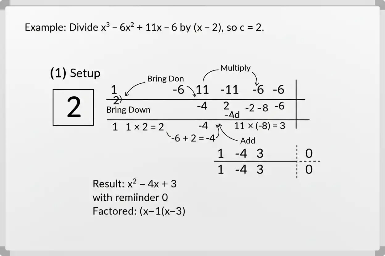
Synthetic division is a shortcut for dividing a polynomial by a linear divisor of the form:
x – c
Instead of repeatedly writing variables and powers as in polynomial long division, synthetic division works primarily with the polynomial’s coefficients.
For example, divide:
x³ – 6x² + 11x – 6
by:
x – 1
Using synthetic division with:
c = 1
produces the quotient:
x² – 5x + 6
with remainder:
0
Therefore:
x³ – 6x² + 11x – 6 = (x – 1)(x² – 5x + 6)
Synthetic division is especially useful for testing factors, reducing polynomial degree, and finding polynomial roots efficiently.
What Is Synthetic Division?
Synthetic division is a compact polynomial-division method that uses coefficients instead of writing every polynomial term repeatedly.
For a polynomial:
P(x)
divided by:
x – c
the division relationship is:
P(x) = (x – c)Q(x) + R
where:
- P(x) is the dividend,
- x – c is the divisor,
- Q(x) is the quotient,
- R is the remainder.
Because the divisor is linear, the remainder is a constant.
Synthetic division performs the same underlying operation as polynomial long division, but it is faster when the divisor has the required linear form.
When Can You Use Synthetic Division?
Standard synthetic division is most directly used when the divisor is:
x – c
Examples include:
x – 3
x + 5
x – 1/2
For:
x + 5
rewrite mentally as:
x – (-5)
so the synthetic value is:
c = -5
Synthetic division is particularly convenient when testing whether a linear expression is a factor of a polynomial.
For more general polynomial divisors such as:
x² + 2x + 1
ordinary polynomial long division is the more general method.
Synthetic Division Formula
The polynomial division identity is:
P(x) = (x – c)Q(x) + R
For a divisor x – c, the remainder satisfies:
R = P(c)
Therefore:
P(x) = (x – c)Q(x) + P(c)
This connection is the basis of the remainder theorem.
If:
P(c) = 0
then:
P(x) = (x – c)Q(x)
and x – c is a factor of the polynomial.
The Synthetic Division Process
Synthetic division follows a repeating pattern:
Bring down → multiply → add → multiply → add
Only the coefficients of the polynomial are used.
Suppose:
P(x) = a₃x³ + a₂x² + a₁x + a₀
and the divisor is:
x – c
Write the coefficients:
a₃, a₂, a₁, a₀
Bring down the first coefficient unchanged. Multiply it by c and place the result under the next coefficient. Add vertically. Repeat until the final column.
The last number is the remainder. The preceding numbers are the coefficients of the quotient.
Example 1: Exact Synthetic Division
Divide:
x³ – 6x² + 11x – 6
by:
x – 1
Since:
x – 1 = x – c
we have:
c = 1
The coefficients are:
1, -6, 11, -6
Bring down the first coefficient:
1
Multiply by 1:
1 × 1 = 1
Add to -6:
-6 + 1 = -5
Multiply:
-5 × 1 = -5
Add to 11:
11 + (-5) = 6
Multiply:
6 × 1 = 6
Add to -6:
-6 + 6 = 0
The synthetic result is:
1, -5, 6 | 0
The first three values are quotient coefficients:
x² – 5x + 6
The final value is the remainder:
R = 0
Therefore:
(x³ – 6x² + 11x – 6)/(x – 1) = x² – 5x + 6
Why the Quotient Degree Drops by One
The dividend in the previous example has degree 3:
x³ – 6x² + 11x – 6
The divisor has degree 1:
x – 1
Therefore the quotient has degree:
3 – 1 = 2
That is why the synthetic output:
1, -5, 6
represents:
x² – 5x + 6
rather than another cubic polynomial.
In general, dividing a degree-n polynomial by a nonzero linear polynomial produces a quotient of degree n – 1.
Example 2: Synthetic Division With a Nonzero Remainder
Divide:
2x³ + 3x² – 5x + 7
by:
x – 2
Use:
c = 2
The coefficients are:
2, 3, -5, 7
Bring down 2.
Multiply:
2 × 2 = 4
Add:
3 + 4 = 7
Multiply:
7 × 2 = 14
Add:
-5 + 14 = 9
Multiply:
9 × 2 = 18
Add:
7 + 18 = 25
The result is:
2, 7, 9 | 25
Therefore the quotient is:
2x² + 7x + 9
and the remainder is:
25
So:
P(x) = (x – 2)(2x² + 7x + 9) + 25
or:
P(x)/(x – 2) = 2x² + 7x + 9 + 25/(x – 2)
Check the Remainder
For division by:
x – 2
the remainder should equal:
P(2)
Evaluate:
P(2) = 2(2³) + 3(2²) – 5(2) + 7
= 16 + 12 – 10 + 7
= 25
This matches the synthetic remainder exactly.
Remainder Theorem
The remainder theorem states that when P(x) is divided by:
x – c
the remainder equals:
P(c)
Symbolically:
R = P(c)
This allows you to find a remainder without carrying out full polynomial division.
For example, find the remainder when:
P(x) = x³ + 2x² – 4x + 5
is divided by:
x – 3
Calculate:
P(3) = 3³ + 2(3²) – 4(3) + 5
= 27 + 18 – 12 + 5
= 38
Therefore the remainder is:
38
Synthetic division would produce the same result.
Factor Theorem
The factor theorem follows directly from the remainder theorem.
If:
P(c) = 0
then:
x – c
is a factor of P(x).
Conversely, if x – c is a factor, then:
P(c) = 0
For example, consider:
P(x) = x³ – 4x² + x + 6
Test:
x – 2
Calculate:
P(2) = 8 – 16 + 2 + 6
P(2) = 0
Therefore:
x – 2
is a factor.
Synthetic division can then find the remaining quotient.
Example 3: Use Synthetic Division to Factor a Cubic
Factor:
x³ – 4x² + x + 6
Knowing x = 2 is a root, divide by:
x – 2
Use coefficients:
1, -4, 1, 6
and:
c = 2
Bring down 1.
Multiply:
1 × 2 = 2
Add:
-4 + 2 = -2
Multiply:
-2 × 2 = -4
Add:
1 – 4 = -3
Multiply:
-3 × 2 = -6
Add:
6 – 6 = 0
The quotient is:
x² – 2x – 3
Factor it:
x² – 2x – 3 = (x – 3)(x + 1)
Therefore:
x³ – 4x² + x + 6 = (x – 2)(x – 3)(x + 1)
The roots are:
x = 2, 3, -1
Once the polynomial is factored, the final values follow from the ordinary rules for solving equations.
Missing Terms in Synthetic Division
Every power must have a coefficient placeholder.
Consider:
x⁴ – 5x² + 4
The polynomial is missing x³ and x terms.
For synthetic division, write the coefficients as:
1, 0, -5, 0, 4
The zero coefficients preserve the correct degree positions.
Failing to include them shifts every later coefficient and produces the wrong quotient.
Example 4: Missing Terms
Divide:
x⁴ – 5x² + 4
by:
x – 1
Use:
c = 1
and coefficients:
1, 0, -5, 0, 4
Bring down:
1
Multiply and add:
0 + 1 = 1
Multiply and add:
-5 + 1 = -4
Multiply and add:
0 – 4 = -4
Multiply and add:
4 – 4 = 0
The result is:
1, 1, -4, -4 | 0
Therefore the quotient is:
x³ + x² – 4x – 4
and:
x⁴ – 5x² + 4 = (x – 1)(x³ + x² – 4x – 4)
Synthetic Division With x + c
Suppose the divisor is:
x + 3
Rewrite it as:
x – (-3)
Therefore the synthetic number is:
-3
This sign change is crucial.
For example, to divide:
x³ + 2x² – 5x – 6
by:
x + 3
use:
c = -3
not c = 3.
Example 5: Divisor x + 3
The coefficients are:
1, 2, -5, -6
Use:
c = -3
Bring down 1.
Multiply:
1(-3) = -3
Add:
2 + (-3) = -1
Multiply:
(-1)(-3) = 3
Add:
-5 + 3 = -2
Multiply:
(-2)(-3) = 6
Add:
-6 + 6 = 0
The quotient is:
x² – x – 2
and the remainder is zero.
Therefore:
x³ + 2x² – 5x – 6 = (x + 3)(x² – x – 2)
Synthetic Division With Fractions
Synthetic division also works when c is fractional.
Suppose the divisor is:
x – 1/2
Use:
c = 1/2
The arithmetic may involve fractions, but the process remains:
bring down → multiply → add
Exact fractions are usually preferable to premature decimal conversion.
What About a Divisor Such as 2x – 3?
Ordinary synthetic division is naturally set up for a monic divisor:
x – c
A divisor:
2x – 3
has the same zero as:
x – 3/2
but those two divisors differ by a factor of 2.
Generalized synthetic methods can account for a non-unit leading coefficient, but ordinary polynomial long division is often clearer when the divisor is not already in the form x – c.
This distinction prevents an otherwise correct synthetic table from being interpreted with the wrong quotient scaling.
Synthetic Division vs Polynomial Long Division
Synthetic division and polynomial long division perform the same basic division operation, but their scope differs.
Synthetic division is compact and efficient for divisors of the form:
x – c
Polynomial long division works with more general polynomial divisors, including:
x² + x – 2
If a divisor is linear and monic, synthetic division is often faster. If it is quadratic or structurally more complicated, long division is the broader method.
Synthetic Division and Polynomial Equations
Synthetic division is especially useful with a higher-degree polynomial equation.
Suppose:
P(x) = 0
and one root r is known.
Then:
x – r
is a factor.
Synthetic division reduces P(x) by that factor and lowers the degree by one.
A cubic may become quadratic, after which factoring or the quadratic formula can find the remaining roots.
Synthetic division therefore assists polynomial solving without replacing the broader theory of polynomial equations.
Synthetic Division After Recognizing a Cube Pattern
Some polynomials already have a specialized factorization.
For example:
x³ – 8
is immediately recognized using sum and difference of cubes:
x³ – 8 = (x – 2)(x² + 2x + 4)
Synthetic division by x – 2 would produce the same quadratic quotient.
When a standard identity is obvious, direct factoring may be faster. Synthetic division becomes especially valuable when a factor is known but the remaining factorization is not immediately visible.
Synthetic Division and Systems of Equations
Synthetic division operates on one polynomial and one linear divisor. It does not solve simultaneous equations.
A system of linear equations instead seeks values satisfying two or more first-degree equations at the same time.
The broader systems of equations topic can also include systems that are not purely linear.
These are different algebraic tasks even though polynomial reductions can occasionally produce equations that later appear inside a larger system.
Synthetic Division vs Line Equations
A line written in standard form of a line has the form:
Ax + By = C
That is a first-degree relationship between x and y.
Synthetic division applies to polynomial division such as:
P(x)/(x – c)
It is not a method for rearranging or graphing a straight-line equation.
Recognizing the structure of the expression tells you which algebraic tool belongs to the problem.
Synthetic Division and Repeated Roots
Suppose:
P(x) = (x – 2)²(x + 3)
The value x = 2 is a repeated root.
Dividing once by:
x – 2
leaves another factor x – 2 in the quotient.
If synthetic division of P(x) by x – 2 gives zero remainder, you can divide the quotient by x – 2 again to test whether the root has higher multiplicity.
Repeated zero remainders reveal repeated factors.
Example 6: Repeated Root
Consider:
P(x) = x³ – 3x² + 4
Test x = 2:
P(2) = 8 – 12 + 4 = 0
Divide by x – 2 using coefficients:
1, -3, 0, 4
Synthetic division gives:
1, -1, -2 | 0
so:
P(x) = (x – 2)(x² – x – 2)
Factor the quotient:
x² – x – 2 = (x – 2)(x + 1)
Therefore:
P(x) = (x – 2)²(x + 1)
The root:
x = 2
has multiplicity 2.
How to Check a Synthetic Division Answer
Use:
Dividend = Divisor × Quotient + Remainder
Suppose synthetic division gives:
Q(x) = x² – 5x + 6
R = 0
for division by x – 1.
Check:
(x – 1)(x² – 5x + 6)
Expand:
x³ – 5x² + 6x – x² + 5x – 6
= x³ – 6x² + 11x – 6
The original dividend is recovered.
For a nonzero remainder, add it after multiplying.
Common Synthetic Division Mistakes
Using the Wrong Sign
For:
x + 4
the synthetic value is:
c = -4
because:
x + 4 = x – (-4)
Forgetting Zero Coefficients
For:
x⁴ – 3x + 2
use:
1, 0, 0, -3, 2
Treating the Last Number as a Quotient Coefficient
The final synthetic value is the remainder.
It is not part of the quotient.
Assigning the Wrong Powers to the Quotient
Dividing a degree-n polynomial by a linear divisor produces a degree-(n – 1) quotient.
Assuming Zero Remainder Means c Is a Factor
If the synthetic value is c and the remainder is zero, the factor is:
x – c
not simply c.
Using Standard Synthetic Division on Any Divisor
The usual shortcut is designed for divisors of the form x – c. More general divisors require long division or an appropriately generalized method.
Skipping Verification
The remainder theorem or the identity:
P(x) = (x – c)Q(x) + R
provides a fast check.
Worked Synthetic Division Example
Divide:
2x⁴ – 3x³ – 5x² + 9x – 3
by:
x – 1
Use:
c = 1
The coefficients are:
2, -3, -5, 9, -3
Bring down:
2
Multiply:
2 × 1 = 2
Add:
-3 + 2 = -1
Multiply:
-1 × 1 = -1
Add:
-5 + (-1) = -6
Multiply:
-6 × 1 = -6
Add:
9 + (-6) = 3
Multiply:
3 × 1 = 3
Add:
-3 + 3 = 0
The result is:
2, -1, -6, 3 | 0
Therefore:
Q(x) = 2x³ – x² – 6x + 3
and:
R = 0
So:
2x⁴ – 3x³ – 5x² + 9x – 3 = (x – 1)(2x³ – x² – 6x + 3)
Because the remainder is zero:
x – 1
is an exact factor.
Frequently Asked Questions
What is synthetic division?
Synthetic division is a compact method for dividing a polynomial by a linear divisor, especially one written as:
x – c
It uses polynomial coefficients rather than repeatedly writing each variable term.
What number do you use for x – 5?
Use:
c = 5
What number do you use for x + 5?
Use:
c = -5
because:
x + 5 = x – (-5)
What is the synthetic division pattern?
The repeating process is:
bring down → multiply → add
Then continue multiplying and adding until the final coefficient is processed.
What does the last number mean?
The last number is the remainder.
How do you identify the quotient?
All synthetic results except the final remainder are coefficients of the quotient, starting one degree below the dividend.
What happens when the remainder is zero?
The divisor is an exact factor of the polynomial.
For division by x – c:
P(c) = 0
What is the remainder theorem?
When P(x) is divided by x – c, the remainder is:
P(c)
What is the factor theorem?
If:
P(c) = 0
then:
x – c
is a factor of P(x).
Why are zero coefficients necessary?
They preserve the position of missing polynomial powers. Without them, the quotient powers and arithmetic become misaligned.
Is synthetic division the same as polynomial long division?
They perform the same type of polynomial division, but synthetic division is a shortcut suited mainly to linear divisors of the form x – c. Polynomial long division handles more general polynomial divisors.
Can synthetic division help find polynomial roots?
Yes. If a candidate root gives zero remainder, its corresponding linear factor can be removed, reducing the polynomial to a lower degree that may be easier to solve.




