


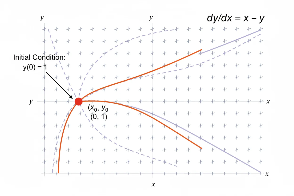
Differential equations are equations that relate an unknown function to one or more of its derivatives. Instead of asking only for a numerical value, they describe how a quantity changes and ask which function follows that rule. A simple example is dy/dx = 3y, which states that the instantaneous rate of change of y is three times its current value. Differential equations can model population growth, cooling, motion, electrical systems, finance, chemical reactions, fluid flow, disease spread, and many other changing processes. Some contain ordinary derivatives with respect to one independent variable, while others contain partial derivatives involving several variables. Their order is determined by the highest derivative appearing in the equation. Solutions may be general families containing arbitrary constants or particular functions selected by initial or boundary conditions. Depending on the equation, a solution may be found exactly, approximated numerically, or studied qualitatively through its behavior.
What Are Differential Equations?
A differential equation is an equation containing an unknown function and at least one derivative of that function.
A basic example is:
dy/dx = 2x
The equation asks for a function y whose derivative equals 2x.
Because:
d/dx[x²] = 2x
one family of solutions is:
y = x² + C
where C is an arbitrary constant.
The constant appears because many functions differing only by a constant have the same derivative.
The broader study of derivatives explains rates of change; differential equations use those rates as relationships that determine unknown functions.
General Form of a Differential Equation
A broad ordinary differential equation can be represented as:
F(x, y, y′, y″, …, y⁽ⁿ⁾) = 0
This notation allows the equation to depend on:
- the independent variable x,
- the unknown function y,
- the first derivative y′,
- the second derivative y″,
- and potentially higher derivatives.
For example:
y″ + 4y′ + 3y = 0
is a second-order differential equation because y″ is the highest derivative present.
Ordinary Differential Equations
An ordinary differential equation, often abbreviated ODE, involves derivatives with respect to a single independent variable.
Examples include:
dy/dx = x + y
and:
y″ + 5y′ + 6y = 0
If y depends only on x, then all derivatives are taken with respect to x.
Many introductory differential equations are ODEs.
Partial Differential Equations
When the unknown function depends on several independent variables and the equation contains partial derivatives, the result is a partial differential equation.
For a function:
u(x, t)
an equation such as:
∂u/∂t = k ∂²u/∂x²
contains derivatives with respect to both position x and time t.
This is structurally different from an ODE because multiple independent directions of change are involved.
Partial derivatives also appear in multivariable concepts such as the directional derivative and gradient.
Order of a Differential Equation
The order of a differential equation is the order of its highest derivative.
For:
dy/dx + 2y = 5
the highest derivative is dy/dx, so this is first order.
For:
d²y/dx² + 3dy/dx + y = 0
the highest derivative is d²y/dx², so this is second order.
For:
y‴ − y′ + 4y = x
the highest derivative is third order.
Therefore, this is a third-order differential equation.
The order influences both the solution method and the number of independent conditions normally required to identify a unique solution.
General and Particular Solutions
A general solution contains arbitrary constants.
For example:
dy/dx = 2x
has the general solution:
y = x² + C
Different values of C give different curves, all satisfying the same differential equation.
A particular solution results when enough additional information determines the arbitrary constants.
Suppose:
y(0) = 5
Substitute x = 0:
5 = 0² + C
Therefore:
C = 5
The particular solution is:
y = x² + 5
Initial Conditions
An initial condition gives the value of the unknown function, and sometimes its derivatives, at a specified input.
For example:
dy/dx = 3y
with:
y(0) = 2
forms an initial value problem.
The differential equation gives the rule of change, while the initial condition identifies the particular solution that begins at the point:
(0, 2)
Without the initial condition, many functions may satisfy the same equation.
Example: Solve dy/dx = 3y
Consider:
dy/dx = 3y
This says that y grows at a rate proportional to its current value.
Separate the variables:
(1/y) dy = 3 dx
Integrate both sides:
∫ (1/y) dy = ∫ 3 dx
This gives:
ln|y| = 3x + C
Exponentiating:
y = Ce³ˣ
where the arbitrary nonzero sign can be absorbed into C. The zero solution is also obtained when C = 0.
So the general solution is:
y = Ce³ˣ
Check the answer by differentiating:
y′ = 3Ce³ˣ
Since:
y = Ce³ˣ
we have:
y′ = 3y
The solution satisfies the original equation.
Example With an Initial Condition
Use the equation:
dy/dx = 3y
with:
y(0) = 2
The general solution is:
y = Ce³ˣ
Apply the initial condition:
2 = Ce⁰
Since:
e⁰ = 1
we obtain:
C = 2
Therefore:
y = 2e³ˣ
This is the unique solution satisfying the given initial condition within the usual setting.
Separable Differential Equations
Some first-order equations can be rearranged so that all y-terms appear with dy and all x-terms appear with dx.
Suppose:
dy/dx = 2xy
Rearrange:
(1/y) dy = 2x dx
Integrate:
∫ (1/y) dy = ∫ 2x dx
Therefore:
ln|y| = x² + C
Exponentiate:
y = Ceˣ²
Differentiate to verify:
y′ = C(2x)eˣ²
= 2xCeˣ²
Since:
y = Ceˣ²
we obtain:
y′ = 2xy
which matches the original equation.
First-Order Linear Differential Equations
A common first-order form is:
dy/dx + P(x)y = Q(x)
This is known as a linear first-order equation.
Its systematic solution typically uses an integrating factor.
The dedicated first-order linear differential equation topic handles that procedure in detail, while the broader differential-equations framework includes many other equation types.
Linear Differential Equations
A differential equation is linear when the unknown function and its derivatives occur to the first power and are not multiplied together.
For example:
y″ + 4y′ + 3y = 0
is linear.
By contrast:
yy′ = x
is nonlinear because y and y′ are multiplied together.
Likewise:
y′ = y² + x
is nonlinear because y appears squared.
The distinction is important because linear equations have structural properties that do not generally hold for nonlinear equations.
Homogeneous and Nonhomogeneous Linear Equations
A linear differential equation may be homogeneous or nonhomogeneous.
For example:
y″ + 4y′ + 3y = 0
is homogeneous because the right-hand side is zero.
By contrast:
y″ + 4y′ + 3y = eˣ
is nonhomogeneous.
The corresponding homogeneous equation often forms an important part of the solution process for a nonhomogeneous problem.
Second-Order Differential Equations
Second-order equations contain a second derivative.
A common form is:
ay″ + by′ + cy = g(x)
where a, b, and c are constants.
For example:
y″ − 5y′ + 6y = 0
is second order.
Because second-order equations involve two levels of differentiation, two independent conditions are typically needed to determine a unique particular solution.
These might be:
y(0) = 2
and:
y′(0) = 1
Such conditions specify both an initial value and an initial rate.
Verifying a Differential Equation Solution
One of the most reliable ways to check an exact solution is to substitute it back into the original equation.
Suppose:
y = 4e²ˣ
and the proposed equation is:
y′ = 2y
Differentiate:
y′ = 8e²ˣ
Calculate the right-hand side:
2y = 2(4e²ˣ)
= 8e²ˣ
Because:
y′ = 2y
the function satisfies the equation.
Verification is especially useful because a small algebraic or sign error during the solution process can otherwise be difficult to notice.
Differential Equations and Integration
Solving simple differential equations frequently requires integration.
For:
dy/dx = f(x)
we can write:
dy = f(x) dx
and integrate:
y = ∫ f(x) dx
For example:
dy/dx = 6x²
gives:
y = 2x³ + C
A definite integral can also express accumulated change when initial values are known.
If:
y′(x) = f(x)
then:
y(b) − y(a) = ∫ₐᵇ f(x) dx
This provides a direct connection between a rate equation and total change.
Differential Equations and Differentials
The notation used in differential equations is closely connected to differentials.
If:
dy/dx = f(x, y)
one may informally rearrange certain separable equations into forms such as:
dy/g(y) = h(x) dx
This arrangement is useful when the variables genuinely separate.
However, not every differential equation can be solved by treating differential symbols as freely rearrangeable algebraic factors. The equation’s structure must support the chosen method.
Exponential Growth and Decay
One of the most important differential-equation models is:
dy/dt = ky
where k is constant.
Its general solution is:
y = Ceᵏᵗ
If:
k > 0
the model represents exponential growth.
If:
k < 0
it represents exponential decay.
The model says that the instantaneous rate of change is proportional to the current amount.
This structure appears in simplified models of population growth, radioactive decay, investment growth, and many other processes.
Example: Exponential Decay
Suppose:
dN/dt = −0.2N
with:
N(0) = 100
The general solution is:
N(t) = Ce⁻⁰·²ᵗ
Using the initial condition:
100 = C
Therefore:
N(t) = 100e⁻⁰·²ᵗ
At t = 5:
N(5) = 100e⁻¹
Since:
e⁻¹ ≈ 0.3679
we obtain:
N(5) ≈ 36.79
The quantity has decreased from 100 to approximately 36.79 after five time units.
Slope Fields
A first-order equation such as:
dy/dx = f(x, y)
specifies a slope at every point where f is defined.
A slope field represents these slopes using short line segments across the coordinate plane.
For example:
dy/dx = y
produces positive slopes where y is positive, negative slopes where y is negative, and zero slopes along y = 0.
Solution curves follow the local directions shown by the slope field.
This provides useful qualitative information even when an exact formula is unavailable.
Numerical Solutions
Not every differential equation has a convenient elementary closed-form solution.
A numerical method can approximate the solution at selected points.
One of the simplest approaches is the Euler method.
For:
y′ = f(x, y)
with step size h, Euler’s update has the form:
yₙ₊₁ = yₙ + h f(xₙ, yₙ)
The current slope estimates how much y changes during the next small step.
Smaller steps often improve accuracy, although they require more calculations and do not eliminate all numerical error.
Euler Method Example
Suppose:
y′ = y
with:
y(0) = 1
Use a step size:
h = 0.1
At the starting point:
x₀ = 0
y₀ = 1
The initial slope is:
f(x₀, y₀) = 1
Euler’s update gives:
y₁ = 1 + 0.1(1)
= 1.1
So:
y(0.1) ≈ 1.1
The exact solution is:
y = eˣ
Therefore:
y(0.1) = e⁰·¹ ≈ 1.10517
The one-step Euler estimate is close but not exact.
Autonomous Differential Equations
An autonomous first-order differential equation has the form:
dy/dt = f(y)
The independent variable does not appear explicitly on the right-hand side.
For example:
dy/dt = y(1 − y)
is autonomous.
Equilibrium solutions occur where:
f(y) = 0
For this example:
y(1 − y) = 0
so the equilibrium values are:
y = 0
and:
y = 1
At an equilibrium, the derivative is zero, so a solution beginning exactly there remains constant.
Equilibrium Solutions
An equilibrium solution is a constant solution that causes the derivative to equal zero.
Consider:
dy/dt = y − 4
Set:
dy/dt = 0
Then:
y − 4 = 0
y = 4
Therefore:
y(t) = 4
is an equilibrium solution.
Equilibria are important when studying the long-term behavior and stability of dynamic systems.
Differential Equations and Rates of Change
Many models begin not with a formula for the quantity itself but with a statement about its rate.
For example:
rate of change = input − output
can lead naturally to a differential equation.
Similarly:
acceleration = applied force / mass
can be incorporated into equations involving second derivatives of position.
This is why differential equations are central whenever the laws governing change are easier to state than the resulting function.
Differential Equations in Motion
If position is:
s(t)
then:
s′(t)
is velocity and:
s″(t)
is acceleration.
Suppose acceleration satisfies:
s″(t) = −9.8
Integrate once:
s′(t) = −9.8t + C₁
Integrate again:
s(t) = −4.9t² + C₁t + C₂
Initial position and velocity determine C₁ and C₂.
A second-order differential equation can therefore encode the motion of an object without stating its position function in advance.
Differential Equations and Directional Change
A basic ODE normally tracks change with respect to one independent variable.
When functions depend on several variables, rates may instead be considered through partial or directional derivatives.
This distinction becomes important in models involving spatial temperature, fluid behavior, potential fields, and other multivariable systems.
The dot product and gradient can also become relevant when expressing directional rates in several dimensions.
Exact Versus Numerical Solutions
An exact solution expresses the function symbolically.
For example:
y = Ce²ˣ
is an exact solution of:
y′ = 2y
A numerical solution instead produces approximate values such as:
y(0.1) ≈ 1.22
y(0.2) ≈ 1.49
depending on the equation and numerical method.
Exact solutions provide formulas valid across intervals, while numerical methods can handle equations for which convenient explicit formulas are unavailable.
Explicit and Implicit Solutions
An explicit solution isolates the dependent variable.
For example:
y = Ceˣ
is explicit.
An implicit solution defines the relationship without isolating y.
For example:
x² + y² = C
can function as an implicit family of solution curves for an appropriate differential equation.
Both forms can be mathematically valid depending on the problem.
What Makes a Differential Equation Difficult?
Difficulty can arise from several sources.
Higher order introduces additional derivatives and conditions. Nonlinearity can prevent techniques available for linear equations. Variable coefficients may complicate standard solution methods. Multiple independent variables lead to partial differential equations. Some equations also have solutions that cannot be represented using elementary functions.
For these reasons, differential equations are classified before a solution method is selected.
Differential Equations and the Calculus Framework
Differential equations combine several core ideas within Calculus & Linear Algebra.
Differentiation describes local change. Integration can recover accumulated quantities. Linear algebra becomes important for systems of equations and higher-dimensional models.
The mathematical tools interact, but each specialist topic retains a distinct purpose: differential equations focus specifically on finding or analyzing functions constrained by derivative relationships.
Common Mistakes
A common mistake is treating every differential equation as though it can be solved by ordinary integration.
For:
dy/dx = 2x
direct integration works easily.
But:
dy/dx = x + y
contains the unknown function on the right-hand side, so simply integrating x + y with respect to x without accounting for y’s dependence on x is not valid.
Another mistake is forgetting arbitrary constants when finding general solutions.
Students may also find a general solution correctly but fail to apply the initial condition needed for the requested particular solution.
Order should be identified from the highest derivative, not from the highest power of x or y.
Finally, an obtained formula should be differentiated and substituted into the original equation whenever practical. Direct verification is one of the most dependable error checks.
Frequently Asked Questions
What is a differential equation?
A differential equation is an equation containing an unknown function and one or more derivatives of that function.
What is a simple example of a differential equation?
A basic example is:
dy/dx = 2x
Its general solution is:
y = x² + C
What is the difference between an ODE and a PDE?
An ordinary differential equation uses derivatives with respect to one independent variable. A partial differential equation involves partial derivatives with respect to multiple independent variables.
What is the order of a differential equation?
The order is the order of the highest derivative appearing in the equation. For example, an equation containing y″ but no higher derivative is second order.
What is a general solution?
A general solution is a family of functions containing one or more arbitrary constants.
What is a particular solution?
A particular solution results when conditions such as initial values determine the arbitrary constants in a general solution.
What is an initial value problem?
It is a differential equation together with one or more conditions specified at an initial point, such as y(0) = 2.
Can all differential equations be solved exactly?
No. Many equations do not have convenient elementary closed-form solutions and must be approximated numerically or analyzed qualitatively.
How do you check a differential equation solution?
Calculate the derivatives required by the equation and substitute the proposed solution and those derivatives back into the original equation. Both sides should agree.
What is a first-order differential equation?
It is an equation whose highest derivative is the first derivative.
Why are differential equations useful?
They describe systems governed by rates of change, making them useful for modeling motion, growth, decay, heat, electrical systems, fluid behavior, biological processes, economics, and many other dynamic phenomena.
What is the relationship between derivatives and differential equations?
A derivative is a rate of change calculated from a known function. A differential equation specifies relationships involving derivatives and asks which unknown functions satisfy those relationships.




