


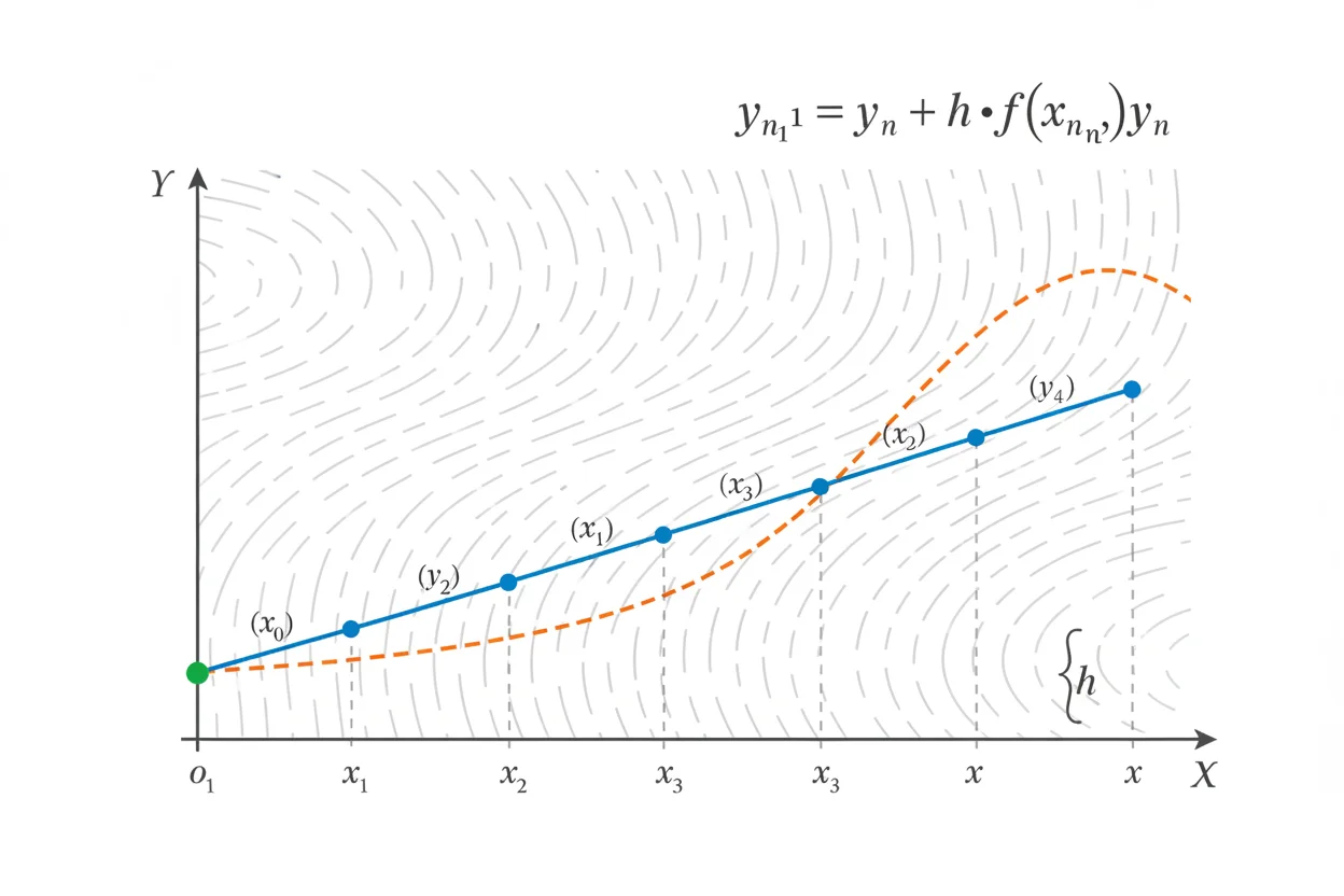
The Euler method is a numerical technique for approximating the solution of a first-order differential equation when an exact solution is unavailable, inconvenient, or unnecessary. Starting from a known initial point, it uses the differential equation to calculate the local slope and then moves a small distance along the corresponding tangent line. The basic update is yₙ₊₁ = yₙ + h f(xₙ, yₙ), where h is the step size and y′ = f(x, y). Each newly estimated point becomes the starting point for the next step. Smaller step sizes generally improve accuracy because the approximation follows the true solution curve more closely, although they require more calculations and do not automatically guarantee stability. The method is especially useful for understanding how numerical solutions to differential equations are constructed. Unlike an analytic solution, Euler’s method usually produces a sequence of approximate values rather than one exact formula for y(x).
What Is the Euler Method?
Suppose a first-order differential equation is:
dy/dx = f(x, y)
and one value of the solution is known:
y(x₀) = y₀
The differential equation tells us the slope of the solution curve at any point:
slope = f(x, y)
Euler’s method uses that slope to make a tangent-line approximation over a small horizontal step h.
Starting from:
(xₙ, yₙ)
the next x-value is:
xₙ₊₁ = xₙ + h
and the next y-value is approximated by:
yₙ₊₁ = yₙ + h f(xₙ, yₙ)
This calculation is repeated as many times as necessary.
The method is based on the same local rate-of-change idea underlying the derivative, but its purpose is numerical approximation rather than symbolic differentiation.
Euler Method Formula
The standard explicit Euler formula is:
yₙ₊₁ = yₙ + h f(xₙ, yₙ)
together with:
xₙ₊₁ = xₙ + h
where:
- xₙ is the current input,
- yₙ is the current approximation,
- h is the step size,
- f(xₙ, yₙ) is the current slope,
- yₙ₊₁ is the next approximate solution value.
Another useful way to see the formula is:
new y ≈ current y + slope × horizontal change
or:
yₙ₊₁ ≈ yₙ + y′ₙh
This is essentially repeated tangent-line approximation.
Why the Euler Method Works
For a differentiable function y(x), a small change in x gives approximately:
Δy ≈ y′ Δx
If:
Δx = h
and:
y′ = f(x, y)
then:
Δy ≈ h f(x, y)
Therefore:
y(x + h) ≈ y(x) + h f(x, y)
This is the local linear idea developed more generally through differentials and linear approximation.
Euler’s method repeatedly applies that approximation along the developing numerical solution.
How to Use Euler’s Method
Given:
y′ = f(x, y)
and:
y(x₀) = y₀
choose a step size h.
At each step, calculate the current slope:
mₙ = f(xₙ, yₙ)
Then calculate the change in y:
Δy ≈ h mₙ
Update y:
yₙ₊₁ = yₙ + h mₙ
Update x:
xₙ₊₁ = xₙ + h
Then repeat with the new point.
The slope must be recalculated after every step because f(x, y) may change as both x and y change.
Example: One Euler Step
Consider:
y′ = x + y
with:
y(0) = 1
and step size:
h = 0.1
The starting values are:
x₀ = 0
y₀ = 1
Find the slope:
f(0, 1) = 0 + 1 = 1
Apply Euler’s formula:
y₁ = 1 + 0.1(1)
y₁ = 1.1
The next x-value is:
x₁ = 0 + 0.1 = 0.1
Therefore:
y(0.1) ≈ 1.1
Example: Several Euler Steps
Continue with:
y′ = x + y
y(0) = 1
h = 0.1
We already found:
(x₁, y₁) = (0.1, 1.1)
At the second point, the slope is:
f(0.1, 1.1) = 0.1 + 1.1
= 1.2
So:
y₂ = 1.1 + 0.1(1.2)
= 1.22
and:
x₂ = 0.2
For the third step:
f(0.2, 1.22) = 0.2 + 1.22
= 1.42
Therefore:
y₃ = 1.22 + 0.1(1.42)
= 1.362
and:
x₃ = 0.3
So the numerical estimates are:
y(0.1) ≈ 1.1
y(0.2) ≈ 1.22
y(0.3) ≈ 1.362
Checking Against the Exact Solution
The equation:
y′ = x + y
can be written:
y′ − y = x
It is a first-order linear differential equation.
Its exact solution satisfying y(0) = 1 is:
y = 2eˣ − x − 1
At:
x = 0.3
the exact value is approximately:
y(0.3) ≈ 1.39972
Euler’s method gave:
y(0.3) ≈ 1.362
The error is approximately:
1.362 − 1.39972 ≈ −0.03772
The approximation is below the exact solution in this example.
Euler Method Table
For the same problem:
| n | xₙ | yₙ | f(xₙ, yₙ) |
|---|---|---|---|
| 0 | 0.0 | 1.000 | 1.000 |
| 1 | 0.1 | 1.100 | 1.200 |
| 2 | 0.2 | 1.220 | 1.420 |
| 3 | 0.3 | 1.362 | — |
A table is useful when several steps must be performed because each new row depends directly on the preceding row.
Example: Exponential Growth
Consider:
y′ = y
with:
y(0) = 1
Use:
h = 0.25
The Euler formula becomes:
yₙ₊₁ = yₙ + 0.25yₙ
or:
yₙ₊₁ = 1.25yₙ
Starting with:
y₀ = 1
we obtain:
y₁ = 1.25
y₂ = 1.5625
y₃ = 1.953125
y₄ = 2.44140625
Therefore:
y(1) ≈ 2.44141
The exact solution is:
y = eˣ
so:
y(1) = e ≈ 2.71828
The Euler estimate is lower by approximately:
2.44141 − 2.71828 ≈ −0.27687
Effect of a Smaller Step Size
Repeat the equation:
y′ = y
with:
y(0) = 1
but use a smaller step size:
h = 0.1
Euler’s recurrence becomes:
yₙ₊₁ = 1.1yₙ
After ten steps:
y₁₀ = 1.1¹⁰
y₁₀ ≈ 2.59374
Compare:
h = 0.25 → y(1) ≈ 2.44141
h = 0.1 → y(1) ≈ 2.59374
exact → y(1) ≈ 2.71828
The smaller step size gives the closer result in this case.
Why Smaller Steps Usually Improve Accuracy
Euler’s method replaces a curved solution segment with a tangent-line segment.
Over a short interval, a smooth curve is usually close to its tangent line.
Over a longer interval, curvature has more opportunity to separate the true solution from the tangent approximation.
Reducing h means the slope is recalculated more frequently, so the polygonal numerical path can adjust more often to the changing differential equation.
This idea connects naturally with the limiting behavior studied through limits, although Euler’s method itself always uses finite step sizes in practical calculations.
Step Size
The step size h controls the horizontal distance between successive estimates.
If:
h > 0
the method moves toward increasing x.
If:
h < 0
it can move backward toward smaller x-values.
For example, to move from:
x = 2
to:
x = 1.5
in five equal steps:
h = (1.5 − 2)/5
h = −0.1
The same Euler formula still applies.
Finding the Number of Steps
Suppose you start at x = a and want to approximate the solution at x = b using constant step size h.
The number of steps is:
N = (b − a)/h
when this quotient is an integer.
For example, from:
x = 0
to:
x = 2
with:
h = 0.25
the number of steps is:
N = 2/0.25
= 8
If the interval is not an exact multiple of h, the final step may need to use a different width.
Example With a Decreasing Solution
Consider:
y′ = −2y
with:
y(0) = 3
and:
h = 0.1
The first slope is:
f(0, 3) = −6
So:
y₁ = 3 + 0.1(−6)
= 2.4
At the next step:
f(0.1, 2.4) = −4.8
Therefore:
y₂ = 2.4 + 0.1(−4.8)
= 1.92
The numerical solution decreases because the derivative is negative.
Example Where the Slope Depends on x and y
Consider:
y′ = x − y
with:
y(0) = 2
and:
h = 0.2
At the initial point:
f(0, 2) = −2
So:
y₁ = 2 + 0.2(−2)
= 1.6
and:
x₁ = 0.2
Now:
f(0.2, 1.6) = 0.2 − 1.6
= −1.4
So:
y₂ = 1.6 + 0.2(−1.4)
= 1.32
At each stage both coordinates must be updated before the next slope is evaluated.
Local Truncation Error
A single Euler step replaces the actual solution curve with its tangent approximation.
For sufficiently smooth solutions, the error introduced during one step is typically proportional to:
h²
in leading order.
This is called local truncation error.
Reducing h therefore makes the error generated during each individual step much smaller.
However, a full calculation contains many steps, so errors can accumulate.
Global Error
The overall error at a fixed endpoint after many Euler steps is generally of order:
h
under standard smoothness assumptions.
This means that, in the asymptotic regime, reducing the step size by roughly half often reduces the overall error by roughly half.
This first-order convergence is why explicit Euler is described as a first-order numerical method.
The exact error behavior still depends on the differential equation, interval, and stability of the computation.
Exact Error Versus Estimated Error
If the exact solution y(x) is known, the error at xₙ can be calculated directly:
errorₙ = yₙ − y(xₙ)
The absolute error is:
|errorₙ| = |yₙ − y(xₙ)|
If the exact solution is unknown, accuracy can instead be investigated by repeating the calculation with smaller step sizes and comparing the numerical results.
Agreement between refinements provides evidence of convergence, although it is not an absolute proof of correctness.
Euler Method and Tangent Lines
At every numerical point:
(xₙ, yₙ)
the differential equation gives a tangent slope:
mₙ = f(xₙ, yₙ)
Euler’s method follows that tangent for horizontal distance h:
y ≈ yₙ + mₙ(x − xₙ)
At:
x = xₙ + h
this becomes:
yₙ₊₁ ≈ yₙ + mₙh
which is exactly the Euler update.
The method can therefore be visualized as a chain of short tangent-line segments.
Euler Method and Slope Fields
A differential equation:
y′ = f(x, y)
assigns a slope to every point where f is defined.
A slope field displays these local directions graphically.
Euler’s method can be viewed as moving through that field: start from the initial condition, follow the current slope for one short step, recalculate the slope, and continue.
This gives a numerical trajectory that approximates a true solution curve.
Euler Method and Initial Value Problems
Euler’s method requires an initial value such as:
y(x₀) = y₀
Without a starting value, the method has no unique point from which to begin.
This mirrors the role of initial conditions in analytic differential equations.
For an equation that admits many solution curves, the initial condition identifies the particular curve Euler’s method is intended to approximate.
Euler Method and Continuity
For straightforward use of Euler’s method, the function:
f(x, y)
should be defined throughout the region visited by the numerical solution.
Regularity such as continuity helps ensure that nearby slopes do not change unpredictably.
Stronger conditions can be needed for uniqueness or rigorous error guarantees.
If f becomes undefined or extremely large near part of the path, numerical behavior may deteriorate.
Euler Method and the Fundamental Theorem of Calculus
If:
y′(x) = f(x, y(x))
then formally:
y(xₙ₊₁) − y(xₙ) = ∫ₓₙˣₙ₊₁ f(x, y(x)) dx
The Fundamental Theorem of Calculus connects the derivative with this accumulated change.
Euler’s method approximates the integral over one small step using the slope at the left endpoint:
∫ₓₙˣₙ₊₁ f(x, y(x)) dx ≈ h f(xₙ, yₙ)
giving:
yₙ₊₁ ≈ yₙ + h f(xₙ, yₙ)
This provides an integration-based interpretation of the same update formula.
Euler Method Versus Exact Integration
A definite integral can calculate exact accumulated change when the relevant integrand is known in a usable form.
Euler’s method is different because, in a general differential equation:
y′ = f(x, y)
the integrand depends on the unknown solution y itself.
The method estimates y and then uses that estimate to determine the next slope.
This recursive dependence is what turns the problem into numerical time-stepping.
Euler Method and Eigenvectors
For a linear vector system:
x′ = Ax
an eigenvector v satisfying:
Av = λv
has especially simple Euler behavior.
If the current state is:
xₙ = cv
then:
xₙ₊₁ = xₙ + hAxₙ
= cv + hcλv
= c(1 + hλ)v
The numerical state remains on the same eigenvector line.
Collections of eigenvectors can therefore help explain the behavior of Euler’s method for linear systems.
Eigenvalues and Numerical Stability
For the scalar test equation:
y′ = λy
Euler’s update is:
yₙ₊₁ = (1 + hλ)yₙ
After n steps:
yₙ = (1 + hλ)ⁿy₀
The corresponding eigenvalues of a matrix system play an analogous role in determining numerical growth or decay along eigenvector directions.
For a decaying exact mode, a poorly chosen h can make the Euler approximation unstable even when the true solution approaches zero.
This shows why step size affects more than accuracy alone.
Stability Example
Consider:
y′ = −10y
The exact solution decays exponentially.
Euler’s update is:
yₙ₊₁ = (1 − 10h)yₙ
If:
h = 0.1
then:
1 − 10h = 0
and one Euler step sends the approximation to zero.
If:
h = 0.3
then:
1 − 10h = −2
so the numerical values alternate signs and double in magnitude:
yₙ₊₁ = −2yₙ
The exact solution decays, but the numerical approximation grows.
This is a stability failure caused by an excessively large step.
Euler Method Versus Analytic Solution
An analytic solution gives a function such as:
y = Ce²ˣ
that can be evaluated throughout an interval.
Euler’s method instead produces values such as:
y₀, y₁, y₂, …
at selected points.
Analytic solutions are preferable when they are available in a useful form and practical to derive.
Numerical solutions become important when the differential equation is too difficult for standard symbolic methods or when only approximate values are required.
Euler Method Versus a Linear Differential Equation Formula
A first-order linear differential equation of the form:
y′ + P(x)y = Q(x)
has an integrating-factor method that can often produce an exact analytic solution.
Euler’s method does not replace that formula. Instead, it approximates the solution numerically from an initial condition.
For an equation where an exact solution is easy to obtain, the exact solution can also be used to evaluate the numerical error of Euler’s method.
Advantages of Euler’s Method
The method is straightforward because each step needs only the current point, the step size, and one evaluation of f(x, y).
It also works for many equations that cannot be solved easily by elementary symbolic techniques.
Its geometric interpretation is clear: repeatedly follow the tangent direction over short distances.
For teaching and basic numerical exploration, these features make Euler’s method particularly useful.
Limitations of Euler’s Method
Euler’s method is only first-order accurate, so high accuracy may require very small steps.
Errors accumulate from one step to the next because every new approximation depends on previous approximations.
A step size that is too large can produce poor accuracy or numerical instability.
The method can also struggle with rapidly changing or stiff differential equations.
More sophisticated numerical methods often achieve substantially better accuracy for a similar amount of interval coverage.
Common Mistakes
A frequent error is calculating every slope from the original point. The slope must be recalculated at the current numerical point:
f(xₙ, yₙ)
Another mistake is updating y but forgetting to update x.
Students may also use:
yₙ₊₁ = yₙ + f(xₙ, yₙ)
and forget the factor h.
The correct formula is:
yₙ₊₁ = yₙ + h f(xₙ, yₙ)
A negative slope should decrease y when h is positive; sign errors can reverse the numerical behavior.
Another common issue is assuming that a smaller step always fixes every numerical problem. Smaller h usually improves Euler accuracy in well-behaved problems, but stability and finite-precision effects still matter.
Finally, Euler values should be reported as approximations unless they happen to coincide exactly with the true solution.
Frequently Asked Questions
What is the Euler method?
The Euler method is a numerical procedure for approximating an initial-value solution of:
y′ = f(x, y)
using repeated tangent-line steps.
What is the Euler method formula?
The main update is:
yₙ₊₁ = yₙ + h f(xₙ, yₙ)
with:
xₙ₊₁ = xₙ + h
What does h mean in Euler’s method?
h is the step size. It controls how far x moves during each numerical step.
How do you start Euler’s method?
You need an initial condition:
y(x₀) = y₀
This provides the first point (x₀, y₀).
Why do you recalculate the slope every step?
Because f(x, y) can change as x and y change. The slope at the previous point generally does not equal the slope at the new point.
Does a smaller h improve Euler’s method?
Usually, for a sufficiently smooth and stable problem, reducing h improves the approximation. It also increases the number of calculations required over the same interval.
Is Euler’s method exact?
Generally no. It is a numerical approximation based on tangent-line steps.
What is the global error order of Euler’s method?
Under standard smoothness assumptions, explicit Euler has first-order global accuracy, commonly expressed as error of order h.
Can Euler’s method be unstable?
Yes. A step size that is too large can cause numerical values to grow or oscillate even when the true solution behaves smoothly or decays.
Can Euler’s method solve nonlinear equations?
Yes. The formula can be applied to nonlinear first-order equations y′ = f(x, y), provided f can be evaluated at the numerical points and the problem is suitable for the method.
Can Euler’s method move backward in x?
Yes. A negative step size allows the calculation to proceed toward smaller x-values.
What is the difference between Euler’s method and an exact differential-equation solution?
An exact solution gives a function satisfying the equation. Euler’s method gives approximate values at discrete points generated from an initial condition.




