


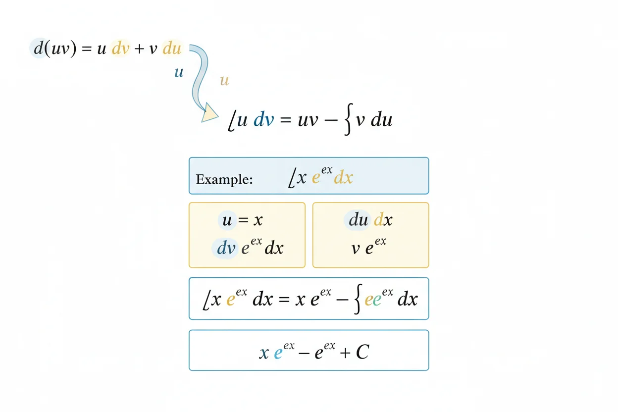
Integration by parts is a technique for integrating products of functions by reversing the product rule for differentiation. Its standard formula is ∫u dv = uv − ∫v du. The method is useful when choosing one factor to differentiate makes it simpler while the other factor is easy to integrate. Common examples include products involving polynomials, logarithms, inverse trigonometric functions, exponentials, and trigonometric functions. Some problems require integration by parts only once, while others require repeated applications. The technique can also solve certain integrals in which the original integral reappears after applying the formula. Unlike integration by substitution, which usually reverses the chain rule, integration by parts specifically reverses the derivative product rule. The key to using it effectively is choosing u and dv so that the remaining integral is simpler than the one you started with.
What Is Integration by Parts?
Integration by parts comes from the product rule for differentiation.
If u and v are differentiable functions, then:
d/dx[uv] = u(dv/dx) + v(du/dx)
Using differential notation:
d(uv) = u dv + v du
Rearrange:
u dv = d(uv) − v du
Integrate both sides:
∫u dv = ∫d(uv) − ∫v du
Therefore:
∫u dv = uv − ∫v du
This is the integration by parts formula.
The technique converts one integral into another. It is worthwhile only when the new integral is easier to evaluate.
Integration by Parts Formula
The standard formula is:
∫u dv = uv − ∫v du
The four pieces are:
u = the function chosen to differentiate
du = derivative of u
dv = the remaining factor, including dx
v = integral of dv
The calculation then follows:
choose u and dv
find du and v
substitute into ∫u dv = uv − ∫v du
evaluate the remaining integral
This method produces an indefinite integral when no bounds are present, so the final answer includes +C.
Basic Example: ∫x eˣ dx
Evaluate:
∫x eˣ dx
Choose:
u = x
dv = eˣ dx
Differentiate u:
du = dx
Integrate dv:
v = eˣ
Apply integration by parts:
∫x eˣ dx = xeˣ − ∫eˣ dx
Since:
∫eˣ dx = eˣ
we obtain:
∫x eˣ dx = xeˣ − eˣ + C
Factor:
∫x eˣ dx = eˣ(x − 1) + C
Check by differentiating:
d/dx[eˣ(x − 1)]
= eˣ(x − 1) + eˣ
= xeˣ
The original integrand is recovered.
Why the Choice of u Matters
Suppose we again have:
∫x eˣ dx
Choosing:
u = x
works well because differentiating x gives:
du = dx
which is simpler.
If instead we choose:
u = eˣ
and:
dv = x dx
then:
du = eˣ dx
and:
v = x²/2
The formula becomes:
x²eˣ/2 − ∫(x²/2)eˣ dx
The remaining integral is more complicated than the original.
A valid mathematical choice is therefore not always a useful choice.
A Practical u-Selection Guideline
A common heuristic is to prefer u from roughly this order:
logarithmic → inverse trigonometric → algebraic → trigonometric → exponential
This is sometimes remembered through variations of the LIATE or ILATE mnemonic.
It is a guideline rather than a theorem.
The real test is whether differentiating u simplifies the expression while dv remains easy to integrate.
Example: ∫x ln x dx
Evaluate:
∫x ln x dx
The logarithm is a natural choice for u:
u = ln x
and:
dv = x dx
Then:
du = 1/x dx
and:
v = x²/2
Apply the formula:
∫x ln x dx = (x²/2)ln x − ∫(x²/2)(1/x) dx
Simplify:
= (x²/2)ln x − (1/2)∫x dx
Integrate:
= (x²/2)ln x − x²/4 + C
Therefore:
∫x ln x dx = (x²/2)ln x − x²/4 + C
for x > 0.
Integrating ln x by Itself
An integral does not need to visibly look like a product before integration by parts can be used.
Consider:
∫ln x dx
Rewrite:
∫1 · ln x dx
Choose:
u = ln x
dv = dx
Then:
du = 1/x dx
v = x
Apply the formula:
∫ln x dx = x ln x − ∫x(1/x) dx
= x ln x − ∫1 dx
Therefore:
∫ln x dx = x ln x − x + C
This is a classic example where multiplying by an implicit factor of 1 reveals the product structure.
Example: Polynomial Times Trigonometric Function
Evaluate:
∫x cos x dx
Choose:
u = x
dv = cos x dx
Then:
du = dx
v = sin x
Apply integration by parts:
∫x cos x dx = x sin x − ∫sin x dx
Since:
∫sin x dx = −cos x
we obtain:
∫x cos x dx = x sin x + cos x + C
Differentiate:
d/dx[x sin x + cos x]
= sin x + x cos x − sin x
= x cos x
The result is correct.
Example: Polynomial Times Sine
Evaluate:
∫x sin x dx
Choose:
u = x
dv = sin x dx
Then:
du = dx
v = −cos x
Apply the formula:
∫x sin x dx = −x cos x − ∫(−cos x) dx
= −x cos x + ∫cos x dx
Therefore:
∫x sin x dx = −x cos x + sin x + C
Signs require particular care when integrating sine.
Repeated Integration by Parts
Higher-degree polynomial factors often require the method more than once.
Consider:
∫x²eˣ dx
First choose:
u = x²
dv = eˣ dx
Then:
du = 2x dx
v = eˣ
So:
∫x²eˣ dx = x²eˣ − 2∫xeˣ dx
We already know:
∫xeˣ dx = xeˣ − eˣ
Therefore:
∫x²eˣ dx = x²eˣ − 2(xeˣ − eˣ) + C
Simplify:
= x²eˣ − 2xeˣ + 2eˣ + C
Factor:
∫x²eˣ dx = eˣ(x² − 2x + 2) + C
Each differentiation of the polynomial lowers its degree until it disappears.
Repeated Example With x³eˣ
For:
∫x³eˣ dx
repeated integration by parts gives:
x³eˣ − 3∫x²eˣ dx
Using the previous result:
= x³eˣ − 3eˣ(x² − 2x + 2) + C
Therefore:
∫x³eˣ dx
= eˣ(x³ − 3x² + 6x − 6) + C
This pattern illustrates why integration by parts is particularly effective when one factor is a polynomial.
Tabular Integration by Parts
When a polynomial is repeatedly differentiated and another function can be repeatedly integrated, a tabular layout can shorten the bookkeeping.
For:
∫x³eˣ dx
successive derivatives of x³ are:
x³
3x²
6x
6
0
Repeated integrals of eˣ remain:
eˣ
The alternating-sign pattern then reconstructs:
eˣ(x³ − 3x² + 6x − 6) + C
Tabular integration is only an organizational shortcut. It is still repeated integration by parts mathematically.
Definite Integration by Parts
For a definite integral, the formula becomes:
∫ₐᵇ u dv = [uv]ₐᵇ − ∫ₐᵇ v du
The boundary term must be evaluated at both endpoints.
For example:
∫₀¹ x eˣ dx
Using:
u = x
dv = eˣ dx
gives:
∫₀¹ x eˣ dx = [xeˣ]₀¹ − ∫₀¹ eˣ dx
Evaluate the first term:
[xeˣ]₀¹ = e
The remaining integral is:
[eˣ]₀¹ = e − 1
Therefore:
∫₀¹ x eˣ dx = e − (e − 1)
= 1
Endpoint Evaluation and the Fundamental Theorem
Once integration by parts produces antiderivative expressions, the Fundamental Theorem Of Calculus handles the endpoint evaluation of a proper definite integral.
For:
∫ₐᵇ u dv
you must preserve:
[uv]ₐᵇ
rather than writing only uv.
Forgetting the boundary evaluation is one of the most common errors when moving from indefinite to definite integration by parts.
Example: ∫₀¹ x ln(1 + x) dx
Evaluate:
∫₀¹ x ln(1 + x) dx
Choose:
u = ln(1 + x)
dv = x dx
Then:
du = 1/(1 + x) dx
v = x²/2
So:
∫₀¹ x ln(1 + x) dx
= [x²ln(1 + x)/2]₀¹ − (1/2)∫₀¹ x²/(1 + x) dx
Divide:
x²/(1 + x) = x − 1 + 1/(1 + x)
Therefore:
= ln 2/2 − (1/2)∫₀¹ [x − 1 + 1/(1 + x)] dx
Evaluate:
∫₀¹ x dx = 1/2
∫₀¹ 1 dx = 1
∫₀¹ 1/(1 + x) dx = ln 2
So:
∫₀¹ x ln(1 + x) dx
= ln 2/2 − (1/2)(1/2 − 1 + ln 2)
= ln 2/2 − 1/2(ln 2 − 1/2)
= ln 2/2 − ln 2/2 + 1/4
Therefore:
∫₀¹ x ln(1 + x) dx = 1/4
Integrals That Return to Themselves
Some integrals produce the original integral again after applying integration by parts twice.
A classic example is:
I = ∫eˣ cos x dx
Choose:
u = cos x
dv = eˣ dx
Then:
du = −sin x dx
v = eˣ
So:
I = eˣ cos x + ∫eˣ sin x dx
Let:
J = ∫eˣ sin x dx
Apply integration by parts again:
u = sin x
dv = eˣ dx
Then:
du = cos x dx
v = eˣ
Thus:
J = eˣ sin x − ∫eˣ cos x dx
J = eˣ sin x − I
Substitute into the first equation:
I = eˣ cos x + eˣ sin x − I
Therefore:
2I = eˣ(cos x + sin x)
and:
I = eˣ(cos x + sin x)/2 + C
The original integral is solved algebraically once it reappears.
Example: ∫eˣ sin x dx
Using the relationship above:
J = eˣ sin x − I
Substitute:
I = eˣ(cos x + sin x)/2
Then:
J = eˣ sin x − eˣ(cos x + sin x)/2
Simplify:
J = eˣ(sin x − cos x)/2 + C
Therefore:
∫eˣ sin x dx = eˣ(sin x − cos x)/2 + C
Differentiation verifies the result.
Integration by Parts and Substitution Together
Some integrals require more than one technique.
For example, an expression might first be simplified by substitution and then require integration by parts, or vice versa.
The broader topic of integrals includes these methods as tools rather than competing definitions.
A useful decision rule is structural: composite-function patterns suggest substitution, while products where one factor simplifies under differentiation suggest parts.
Integration by Parts Versus Substitution
Consider:
∫2x(x² + 1)⁵ dx
This is naturally handled through substitution because 2x is the derivative of x² + 1.
By contrast:
∫xeˣ dx
has no inner function whose derivative appears as the remaining factor. Differentiating x makes the product simpler, so integration by parts is the more natural choice.
The two methods can be summarized conceptually as:
substitution reverses the chain rule
integration by parts reverses the product rule
This distinction helps avoid unnecessary algebra.
Integration by Parts and the Chain Rule
Although integration by parts comes from the product rule, the chain rule can still appear inside individual steps.
For example, integrating:
e^(2x)
as part of dv gives:
e^(2x)/2
because differentiating the exponent contributes a factor of 2.
Thus selecting the main integration technique does not eliminate the need for ordinary derivative and antiderivative rules inside the calculation.
Integration by Parts With Inverse Trigonometric Functions
Consider:
∫arctan x dx
Rewrite:
∫1 · arctan x dx
Choose:
u = arctan x
dv = dx
Then:
du = 1/(1 + x²) dx
v = x
Apply the formula:
∫arctan x dx
= x arctan x − ∫x/(1 + x²) dx
The remaining integral is suited to substitution.
Let:
w = 1 + x²
dw = 2x dx
Then:
∫x/(1 + x²) dx = (1/2)ln(1 + x²)
Therefore:
∫arctan x dx
= x arctan x − (1/2)ln(1 + x²) + C
This example shows two integration techniques working in sequence.
Integration by Parts With Polynomial Powers
For:
∫xⁿeˣ dx
where n is a nonnegative integer, repeated integration by parts progressively reduces:
xⁿ → nxⁿ⁻¹ → n(n − 1)xⁿ⁻² → …
until the polynomial disappears.
This is analogous to repeated use of the power rule during differentiation.
The exponential factor remains easy to integrate throughout, which makes the method efficient.
Reduction Formulas
Repeated integration by parts can produce recurrence relationships between integrals.
For example, define:
Iₙ = ∫xⁿeˣ dx
Choose:
u = xⁿ
dv = eˣ dx
Then:
du = nxⁿ⁻¹ dx
v = eˣ
Therefore:
Iₙ = xⁿeˣ − nIₙ₋₁
This is a reduction formula.
It expresses a harder integral in terms of a similar integral with a lower power.
Integration by Parts and Improper Integrals
Integration by parts can also appear inside an improper integral, but the improper endpoint must still be handled using a limit.
Consider:
∫₀∞ xe^(−x) dx
Write:
lim as b → ∞ of ∫₀ᵇ xe^(−x) dx
For the finite integral choose:
u = x
dv = e^(−x) dx
Then:
du = dx
v = −e^(−x)
So:
∫₀ᵇ xe^(−x) dx
= [−xe^(−x)]₀ᵇ + ∫₀ᵇ e^(−x) dx
This becomes:
−be^(−b) + 1 − e^(−b)
As:
b → ∞
both exponential terms approach zero.
Therefore:
∫₀∞ xe^(−x) dx = 1
The integration-by-parts step does not replace the convergence limit.
Limits Inside the Method
The required behavior in an improper problem depends on a limit.
For example:
lim as b → ∞ of be^(−b) = 0
This limit justifies the disappearance of the boundary term in the preceding example.
Knowing the antiderivative alone is insufficient when a bound is infinite or an integrand is unbounded.
Integration by Parts and Partial Fractions
A rational function is not automatically a good integration-by-parts candidate.
If numerator and denominator are polynomial expressions and the denominator factors, partial fraction integration may be more appropriate.
For example:
∫1/[(x + 1)(x + 2)] dx
is naturally decomposed into simpler rational terms rather than handled by parts.
Technique selection should follow algebraic structure.
Integration by Parts and Differential Equations
Integration by parts can appear when solving or analyzing differential equations, especially when integral identities or transform methods arise.
However, it is an integration technique rather than a differential-equation solution category.
A first-order linear differential equation primarily uses an integrating factor, although evaluating the resulting integral may occasionally require integration by parts.
Integration by Parts in Multivariable Calculus
The same product-rule principle extends beyond ordinary one-variable integration.
In multivariable calculus, related identities connect derivatives and integrals over higher-dimensional domains.
The elementary formula:
∫u dv = uv − ∫v du
is the one-variable form most commonly used for direct antiderivative calculations.
Keeping that scope clear avoids confusing it with double, line, or surface integration procedures.
When Not to Use Integration by Parts
Do not use integration by parts simply because an integrand contains two visible factors.
For:
∫2x(x² + 1)⁵ dx
substitution is much shorter.
For:
∫x² dx
the ordinary power rule is enough.
For:
∫1/(x² − 1) dx
algebra and partial fractions are more natural.
A good integration method reduces complexity. If applying parts makes the remaining integral more difficult without revealing a useful cycle or recurrence, reconsider the choice.
Common Mistakes
A frequent mistake is forgetting the minus sign:
∫u dv = uv − ∫v du
not:
uv + ∫v du
Another error is choosing dv that cannot be integrated conveniently.
Students may also forget to include all remaining factors and dx inside dv.
For definite integrals, the term:
uv
must be evaluated at both endpoints.
Repeated applications require careful sign management, especially with trigonometric functions.
When the original integral returns after several steps, it should be collected algebraically rather than treated as a failure.
Finally, always differentiate an indefinite result when practical. This quickly reveals sign errors and missing factors.
Frequently Asked Questions
What is the integration by parts formula?
The standard formula is:
∫u dv = uv − ∫v du
Where does integration by parts come from?
It is derived from the product rule for differentiation:
d(uv) = u dv + v du
When should I use integration by parts?
It is especially useful for products where one factor becomes simpler when differentiated and the other factor is easy to integrate.
How do I choose u?
Logarithmic and inverse trigonometric functions are often good choices, followed by algebraic functions. The best choice is the one that simplifies the remaining integral.
Can integration by parts be used more than once?
Yes. Polynomial-exponential and polynomial-trigonometric products often require repeated applications.
Can I use integration by parts on ln x?
Yes. Rewrite it as:
1 · ln x
then choose ln x as u and dx as dv.
What is the definite integration-by-parts formula?
∫ₐᵇ u dv = [uv]ₐᵇ − ∫ₐᵇ v du
What if the original integral appears again?
Collect it algebraically on one side and solve for it. Integrals such as ∫eˣcos x dx are standard examples.
What is the difference between integration by parts and substitution?
Integration by parts reverses the product rule. Substitution primarily reverses the chain rule.
Does integration by parts always make an integral easier?
No. A poor choice of u and dv can make the remaining integral more complicated.
Can integration by parts be used with improper integrals?
Yes, but first work on a proper finite interval and then take the required limit. Convergence still has to be established.
How can I check an integration-by-parts answer?
Differentiate the final antiderivative. It should reproduce the original integrand exactly.




