


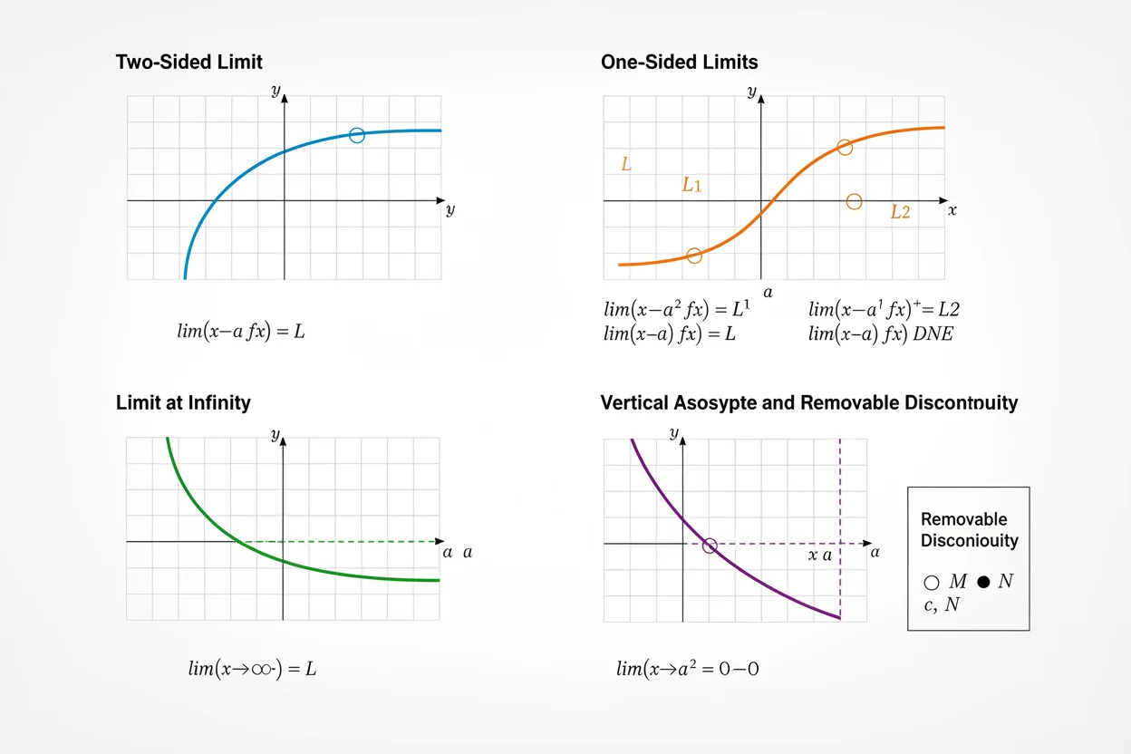
Limits describe how functions behave as inputs approach particular values, approach from one side, or grow without bound. They provide the language needed to discuss behavior that may not be captured by direct function values alone. Limits include ordinary two-sided limits, left-hand and right-hand limits, infinite limits, limits at infinity, limits of sequences, and limiting expressions that require algebraic or comparative analysis. A two-sided limit exists only when the corresponding one-sided limits agree. A finite limit can exist even when a function is undefined at the target point, while an assigned function value can exist even when the nearby limit fails. Limit laws make many calculations algebraic, but indeterminate forms such as 0/0 require additional work. Limits also provide the foundation for continuity, derivative definitions, tangent approximations, improper integration, and rigorous accumulation. Understanding the different kinds of limits is therefore more important than memorizing a single evaluation technique.
What Are Limits?
Limits answer questions of the form:
What does this expression approach?
A typical finite limit is written:
limₓ→ₐ f(x) = L
This means that f(x) approaches L as x approaches a.
The singular limit calculation focuses on determining one such value. The broader concept of limits includes several kinds of approach behavior, rules for existence, asymptotic cases, and the way limiting processes support the rest of calculus.
For example:
limₓ→₂ x² = 4
because values of x close to 2 produce values of x² close to 4.
Why Limits Are Needed
Suppose:
f(x) = (x² − 4)/(x − 2)
At:
x = 2
the function is undefined.
Yet for x ≠ 2:
f(x) = x + 2
So nearby values approach:
4
Therefore:
limₓ→₂ f(x) = 4
Limits let us describe this nearby behavior even though there is no original function value at the target point.
Without this distinction, holes, asymptotes, instantaneous rates, and infinite processes would be difficult to describe precisely.
Main Types of Limits
In elementary calculus, the most common categories are:
- finite two-sided limits,
- one-sided limits,
- infinite limits,
- limits at infinity,
- sequence limits,
- and limits involving indeterminate forms.
Each category asks about an approach process, but the input and output behavior differ.
These distinctions determine which calculation or existence test is appropriate.
Finite Two-Sided Limits
A standard two-sided limit has the form:
limₓ→ₐ f(x) = L
It requires the function to approach the same number L from both sides of a.
For example:
limₓ→₃ (x² − 1) = 8
because direct substitution gives:
3² − 1 = 8
and the polynomial behaves continuously near x = 3.
Left-Hand Limits
A left-hand limit asks what happens as x approaches a using values smaller than a.
Conceptually:
x → a from the left
For example, define:
f(x) = 2x + 1 for x < 3
Then:
lim as x → 3 from the left of f(x)
is:
2(3) + 1 = 7
The point x = 3 itself need not belong to this branch.
Right-Hand Limits
A right-hand limit asks what happens as x approaches a using values larger than a.
Suppose:
f(x) = x² for x ≥ 3
Then:
lim as x → 3 from the right of f(x) = 9
One-sided limits are essential around jump discontinuities, domain endpoints, vertical asymptotes, and piecewise functions.
Two-Sided Limit Existence
A two-sided limit exists if and only if the left-hand and right-hand limits both exist and are equal.
If:
left-hand limit = L
and:
right-hand limit = L
then:
limₓ→ₐ f(x) = L
If the two one-sided values differ, the ordinary two-sided limit does not exist.
This criterion is one of the most important structural rules for limits.
Example: Matching Sides
Define:
f(x) = x² for x < 1
f(x) = 2x − 1 for x ≥ 1
From the left:
x² → 1
From the right:
2x − 1 → 1
Therefore:
limₓ→₁ f(x) = 1
The assigned value is also:
f(1) = 1
so the function is continuous there.
Example: Mismatched Sides
Define:
f(x) = x + 2 for x < 1
f(x) = x + 5 for x ≥ 1
The left-hand limit is:
3
The right-hand limit is:
6
Because:
3 ≠ 6
the two-sided limit does not exist.
No choice of f(1) can make the nearby left and right behaviors agree.
Limits and Function Values
Three possibilities are important.
A limit and function value can both exist and be equal.
They can both exist but be different.
A limit can exist while the function value does not.
For example, define:
f(x) = x² for x ≠ 2
and:
f(2) = 10
Then:
limₓ→₂ f(x) = 4
but:
f(2) = 10
This distinction forms the basis of continuity.
Limits and Continuity
A function is continuous at x = a when:
f(a) exists
limₓ→ₐ f(x) exists
limₓ→ₐ f(x) = f(a)
Thus limits characterize whether nearby function behavior connects smoothly to the actual function value.
If the finite limit exists but f(a) is missing or incorrectly assigned, the discontinuity may be removable.
If the one-sided limits differ, changing a single point cannot restore continuity.
Direct Substitution and Continuous Functions
Many limits are simple because common functions are continuous throughout their domains.
For example:
limₓ→₄ (x³ − 2x)
is:
4³ − 2(4)
= 64 − 8
= 56
Similarly:
limₓ→₉ √x = 3
because the square-root function is continuous at 9.
Direct substitution works whenever the function’s structure and domain permit it.
Limit Laws
Suppose:
limₓ→ₐ f(x) = L
and:
limₓ→ₐ g(x) = M
Then, under the usual conditions:
limₓ→ₐ [f(x) + g(x)] = L + M
limₓ→ₐ [f(x) − g(x)] = L − M
limₓ→ₐ [cf(x)] = cL
limₓ→ₐ [f(x)g(x)] = LM
and:
limₓ→ₐ f(x)/g(x) = L/M
provided:
M ≠ 0
Powers and suitable roots can also pass through limits.
These rules let complex expressions be decomposed into simpler limit components.
Example Using Limit Laws
Evaluate:
limₓ→₂ [(x² + 1)(3x − 4)]
Find the separate limits:
x² + 1 → 5
and:
3x − 4 → 2
By the product rule:
limit = 5 × 2
= 10
Direct substitution gives the same answer, but the example illustrates how the laws combine component limits.
Indeterminate Forms
Some substitutions produce expressions that do not determine a limit directly.
Common indeterminate forms include:
0/0
∞/∞
0 · ∞
∞ − ∞
and certain exponential forms such as:
1^∞
The word indeterminate means the visible form alone does not identify the answer.
Different expressions with the same apparent form can have completely different limits.
Further simplification or analysis is required.
Why 0/0 Is Indeterminate
Compare:
x/x
as x → 0.
For x ≠ 0:
x/x = 1
so the limit is:
1
Now consider:
x²/x
For x ≠ 0:
x²/x = x
so the limit is:
0
And:
x/x² = 1/x
does not have a finite two-sided limit as x → 0.
All three expressions appear as 0/0 under direct substitution, yet their limiting behaviors are different.
Therefore 0/0 cannot itself be treated as an answer.
Factoring Limits
Evaluate:
limₓ→₄ (x² − 16)/(x − 4)
Direct substitution gives:
0/0
Factor:
x² − 16 = (x − 4)(x + 4)
For x ≠ 4:
(x² − 16)/(x − 4) = x + 4
Therefore:
limₓ→₄ (x² − 16)/(x − 4) = 8
Factoring removes a removable algebraic obstruction while preserving the behavior near the target.
Rationalizing Limits
Consider:
limₓ→₀ [√(1 + x) − 1]/x
Multiply by the conjugate:
√(1 + x) + 1
The expression becomes:
[(1 + x) − 1]/[x(√(1 + x) + 1)]
= x/[x(√(1 + x) + 1)]
For x ≠ 0:
= 1/[√(1 + x) + 1]
Therefore:
limit = 1/2
Rationalization is especially useful when a radical difference produces 0/0.
Trigonometric Limits
A foundational trigonometric result is:
limₓ→₀ sin x/x = 1
with x measured in radians.
From it, many related limits follow.
For example:
limₓ→₀ sin(5x)/x
Rewrite:
sin(5x)/x = 5 · sin(5x)/(5x)
As x → 0:
5x → 0
Therefore:
limit = 5 · 1
= 5
Recognizing the standard trigonometric pattern can avoid lengthy algebra.
The Squeeze Theorem
Suppose:
g(x) ≤ f(x) ≤ h(x)
near x = a.
If:
limₓ→ₐ g(x) = L
and:
limₓ→ₐ h(x) = L
then:
limₓ→ₐ f(x) = L
This result is particularly valuable when f oscillates or is difficult to simplify directly.
The outer functions squeeze the middle expression toward one unavoidable value.
Squeeze Example
For x ≠ 0:
−1 ≤ sin(1/x) ≤ 1
Multiply by |x|:
−|x| ≤ |x|sin(1/x) ≤ |x|
Both outside expressions approach:
0
as x → 0.
Therefore:
limₓ→₀ |x|sin(1/x) = 0
The oscillation remains, but its amplitude collapses toward zero.
Infinite Limits
An infinite limit describes output becoming arbitrarily large in magnitude near a finite input.
For example:
limₓ→₀ 1/x² = ∞
The function does not approach a finite real number.
Instead, both sides grow positively without bound.
The graph has a vertical asymptote:
x = 0
Infinite-limit notation describes behavior rather than assigning infinity as an ordinary function value.
Different Signs From Different Sides
Consider:
1/x
near x = 0.
From the right:
1/x → ∞
From the left:
1/x → −∞
Because the behaviors differ, there is no single same-sign two-sided infinite limit.
This one-sided analysis is essential around vertical asymptotes.
Limits at Infinity
A limit at infinity examines long-run behavior.
For example:
limₓ→∞ 1/x² = 0
and:
limₓ→−∞ 1/x² = 0
The graph approaches the horizontal line:
y = 0
Such limits help identify horizontal asymptotes and dominant growth behavior.
Polynomial Growth at Infinity
Consider:
limₓ→∞ (2x³ − x)
The leading term:
2x³
dominates.
Therefore the expression grows without bound:
2x³ − x → ∞
As:
x → −∞
the cubic term becomes negative without bound:
2x³ − x → −∞
Leading terms usually determine polynomial behavior at large magnitude.
Rational Limits at Infinity
For:
(aₙxⁿ + lower terms)/(bₘxᵐ + lower terms)
compare the degrees n and m.
If:
n < m
the limit as x → ±∞ is usually:
0
If:
n = m
the finite limit is the ratio:
aₙ/bₘ
If:
n > m
the function generally does not approach a finite horizontal limit.
For example:
limₓ→∞ (5x² + 1)/(2x² − 3x) = 5/2
Horizontal Asymptotes
If:
limₓ→∞ f(x) = L
or:
limₓ→−∞ f(x) = L
then:
y = L
is a horizontal asymptote in that direction.
A function may cross its horizontal asymptote. The asymptote describes long-run approach, not a barrier the graph cannot touch.
A function can also have different horizontal asymptotes as x → ∞ and x → −∞.
Vertical Asymptotes
If:
f(x) → ±∞
as x approaches a from at least one side, then:
x = a
is typically a vertical asymptote.
For example:
f(x) = 1/(x − 2)
has vertical asymptote:
x = 2
because the denominator approaches zero and the function grows without bound in opposite directions on the two sides.
Limits of Sequences
Limits also apply to sequences.
If:
aₙ = 1/n
then:
aₙ → 0 as n → ∞
because the terms become arbitrarily close to zero as the index grows.
A sequence has a finite limit L if its terms eventually become and remain arbitrarily close to L.
This discrete version of limiting behavior parallels function limits at infinity.
Example of a Sequence Limit
Consider:
aₙ = (2n + 1)/n
Rewrite:
aₙ = 2 + 1/n
As:
n → ∞
we have:
1/n → 0
Therefore:
aₙ → 2
The sequence approaches 2 without needing any term to equal exactly 2.
Divergent Sequences
Not every sequence has a limit.
For example:
aₙ = (−1)ⁿ
alternates:
−1, 1, −1, 1, …
It never settles near one number.
Therefore the sequence diverges.
Similarly:
aₙ = n
grows without bound and has no finite real limit.
Formal Idea Behind Limits
Informally, saying:
limₓ→ₐ f(x) = L
means that f(x) can be made as close to L as desired by requiring x to be sufficiently close to a, without requiring x = a.
The rigorous formulation uses positive tolerances traditionally denoted ε and δ.
For every:
ε > 0
there must exist:
δ > 0
such that whenever:
0 < |x − a| < δ
we have:
|f(x) − L| < ε
This definition makes the phrase “approaches” mathematically precise.
Simple ε–δ Example
Consider:
f(x) = 2x
and show conceptually that:
limₓ→₃ 2x = 6
We want:
|2x − 6| < ε
Factor:
|2(x − 3)| < ε
So:
2|x − 3| < ε
It is enough to require:
|x − 3| < ε/2
Therefore choosing:
δ = ε/2
guarantees the desired output closeness.
This illustrates how input and output tolerances are connected.
Limits and Derivatives
A derivative is a specific kind of limit:
f′(a) = lim as h → 0 of [f(a + h) − f(a)]/h
The fraction measures average change over an interval of width h.
The limiting process lets h shrink toward zero, producing instantaneous change.
Thus limits are not merely one topic before differentiation; they are embedded in the definition of the derivative itself.
Limits and Continuity of Derivatives
For a derivative to exist at a point, the corresponding difference-quotient limit must exist as a finite value.
A function can be continuous without being differentiable.
For example:
f(x) = |x|
is continuous at zero, but its difference quotient approaches different slopes from the two sides.
Therefore the derivative limit at zero does not exist.
This illustrates how different limiting conditions create distinct calculus properties.
Limits and Linear Approximation
A linear approximation uses:
f(x) ≈ f(a) + f′(a)(x − a)
near x = a.
The approximation is justified by a limiting idea: the error relative to the input displacement becomes negligible as x approaches a for a differentiable function.
The tangent line therefore becomes an increasingly accurate local model at sufficiently small scales.
Limits give mathematical meaning to the phrase “locally linear.”
Limits and Differentials
The relationship:
dy = f′(x)dx
from differentials expresses the first-order local change predicted from a derivative.
Because f′ itself is defined by a limit, the differential approximation ultimately rests on limiting behavior.
For small Δx:
Δy ≈ dy
and the approximation improves locally as the displacement shrinks under suitable smoothness conditions.
Limits and Integrals
A definite integral can be constructed as a limit of sums.
Partition:
[a, b]
into small intervals and form:
Σ f(xᵢ*)Δxᵢ
As the partition becomes finer, the sums approach:
∫ₐᵇ f(x) dx
when the relevant integrability conditions hold.
Thus integrals use limits to turn finite approximating sums into exact accumulated quantities.
Limits and Improper Integrals
An improper integral uses limits explicitly.
For example:
∫₁∞ f(x) dx
means:
lim as b → ∞ of ∫₁ᵇ f(x) dx
A singular endpoint is handled similarly through a one-sided limit.
The improper integral converges only when the required limiting values are finite.
This is one of the clearest applications of limits outside derivative definitions.
Limits and Integration by Substitution
Integration by substitution changes the variable of integration.
When the original integral has ordinary finite bounds, those bounds can be transformed directly.
When a bound involves infinity or approaches a singularity, its transformed value must be determined by limiting behavior.
For example, if:
u = x² + 1
then:
x → ∞
implies:
u → ∞
This ensures the transformed improper integral represents the same asymptotic domain.
Limits and Integration by Parts
Integration by parts reverses the product rule.
In an improper integral, boundary terms produced by integration by parts often require their own limits.
For example:
be^(−b)
approaches zero as:
b → ∞
even though b itself grows without bound.
Recognizing which factor dominates is therefore essential when evaluating boundary terms.
Limits and Line Integrals
A line integral accumulates a quantity along a curve.
Its theoretical construction can be viewed through limits of sums over shorter and shorter pieces of the path.
In practical calculations, a parameterization usually converts the path integral into an ordinary definite integral.
Limits therefore provide the foundation while the parameterized integral provides the computational form.
Limits and the Fundamental Theorem
The Fundamental Theorem Of Calculus connects differentiation and integration after both have been established through limiting ideas.
The derivative uses a limit of difference quotients.
The integral can use a limit of sums.
The theorem then shows that under suitable conditions these apparently different limiting processes are inverse operations.
This connection is one of the central organizing ideas of calculus.
Limits and Differential Equations
Differential equations contain derivatives, so limits are built indirectly into their meaning.
Numerical methods also rely on smaller step sizes to approximate continuous evolution.
For instance, the Euler method uses finite tangent steps; examining what happens as step sizes shrink helps explain convergence toward an exact solution under suitable conditions.
The limit concept therefore supports both analytic and numerical differential-equation theory.
Limits in Multivariable Calculus
In multivariable calculus, approaching a point becomes more demanding because infinitely many paths can lead to the same location.
For:
f(x, y)
a two-variable limit:
(x, y) → (a, b)
must approach the same output regardless of the path taken, if the full limit is to exist.
Agreement along a few paths does not prove existence.
However, finding two paths with different limiting values is enough to prove that the limit does not exist.
Path Dependence Example
Consider:
f(x, y) = x²/(x² + y²)
as:
(x, y) → (0, 0)
Along:
y = 0
we obtain:
f(x, 0) = 1
so the path limit is:
1
Along:
x = 0
we obtain:
f(0, y) = 0
so the path limit is:
0
Because two paths produce different values, the full two-variable limit does not exist.
This illustrates why multidimensional limits require path-independent approach behavior.
Limits and Gradient Calculations
A gradient is built from partial derivatives, and partial derivatives themselves are one-dimensional limiting rates along coordinate directions.
However, existence of partial derivatives does not automatically establish full differentiability of a multivariable function.
The full local behavior may depend on more than coordinate-direction limits.
This distinction becomes important when moving from elementary one-variable limits to higher-dimensional calculus.
Limits and Asymptotic Comparison
Limits can compare the long-run size of functions.
If:
limₓ→∞ f(x)/g(x) = 1
then f and g have the same leading asymptotic behavior.
For example:
f(x) = x² + 3x
and:
g(x) = x²
Then:
f(x)/g(x) = 1 + 3/x
As x → ∞:
1 + 3/x → 1
So x² is the dominant long-run term.
This type of comparison helps simplify rational expressions and growth-rate analysis.
Common Mistakes With Limits
A frequent mistake is confusing a limit with a function value. Limits describe approach behavior and can exist even when the value at the point is missing.
Another error is declaring that 0/0 equals zero. It is an indeterminate form.
For two-sided limits, checking only one direction is insufficient.
Infinity is not an ordinary number and should not be substituted as though it were a finite endpoint.
When evaluating rational functions at infinity, lower-degree terms should not be allowed to obscure the dominant powers.
Students may also assume that matching limits along two paths proves a multivariable limit exists. It does not; all possible approaches must be consistent.
Finally, limit laws should only be applied when their required component limits and denominator conditions are satisfied.
Frequently Asked Questions
What are limits in calculus?
Limits describe the values functions or sequences approach as their inputs or indices approach specified values or infinity.
What is the basic limit notation?
limₓ→ₐ f(x) = L
means f(x) approaches L as x approaches a.
What types of limits are there?
Common types include two-sided limits, left-hand limits, right-hand limits, infinite limits, limits at infinity, sequence limits, and multivariable limits.
When does a two-sided limit exist?
It exists when the left-hand and right-hand limits both exist and are equal.
Can limits exist when functions are undefined?
Yes. A function can be undefined at the target point while its nearby values approach one finite number.
What is an indeterminate form?
It is a form such as 0/0 or ∞/∞ that does not determine a limiting value without further analysis.
What is the difference between an infinite limit and a limit at infinity?
An infinite limit describes output growing without bound as the input approaches a finite point. A limit at infinity describes function behavior as the input itself grows without bound.
How are limits related to continuity?
Continuity at a requires:
limₓ→ₐ f(x) = f(a)
together with existence of both sides and the function value.
How are limits related to derivatives?
Derivatives are defined as limits of difference quotients.
How are limits related to integrals?
Definite integrals can be defined as limits of sums, while improper integrals use limits to handle infinite bounds and singularities.
Can a multivariable limit depend on the path?
If different paths toward the same point produce different values, the full multivariable limit does not exist.
Why are limits important?
They provide the precise mathematical framework for instantaneous change, continuity, infinite processes, local approximation, integral accumulation, and asymptotic behavior.




