


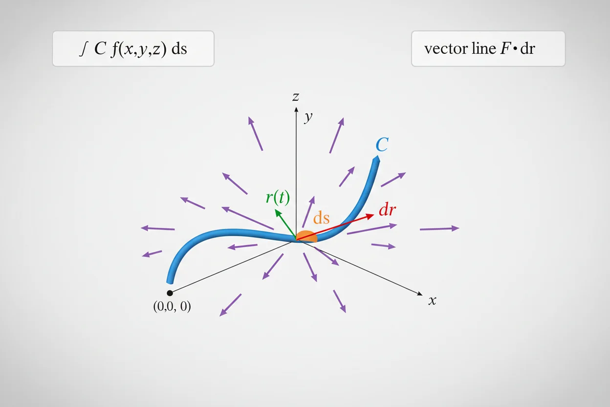
A line integral accumulates a quantity along a curve rather than across an ordinary straight interval or two-dimensional region. For a scalar field f, the line integral ∫꜀ f ds weights the field by small elements of arc length along the path. For a vector field F, the line integral ∫꜀ F · dr measures the component of the field acting along the direction of motion and often represents work or circulation. In practice, the curve is parameterized as r(t), converting the line integral into an ordinary single-variable definite integral. Scalar line integrals use ds = |r′(t)|dt, while vector line integrals use dr = r′(t)dt. The value can depend on the shape of the path, and a vector line integral can also change sign when the path orientation is reversed. Certain gradient fields are path independent, allowing their line integrals to be calculated from endpoint values alone. Line integrals therefore connect curves, vectors, derivatives, and ordinary integration within multivariable calculus.
What Is a Line Integral?
An ordinary integral such as:
∫ₐᵇ f(x) dx
accumulates values along an interval on the x-axis.
A line integral generalizes this idea to a curve C.
Instead of moving only from x = a to x = b, we may follow a curved path through two- or three-dimensional space.
There are two common forms:
∫꜀ f ds
for a scalar field, and:
∫꜀ F · dr
for a vector field.
Although both are line integrals, they accumulate different kinds of quantities.
The scalar form weights a scalar value by distance traveled along the curve. The vector form measures how much a vector field points along the path.
Scalar Line Integral Formula
Suppose a curve C is parameterized by:
r(t) = (x(t), y(t))
for:
a ≤ t ≤ b
The arc-length element is:
ds = |r′(t)|dt
where:
r′(t) = (x′(t), y′(t))
and:
|r′(t)| = √[x′(t)² + y′(t)²]
Therefore:
∫꜀ f ds = ∫ₐᵇ f(x(t), y(t))|r′(t)|dt
In three dimensions:
r(t) = (x(t), y(t), z(t))
and:
|r′(t)| = √[x′(t)² + y′(t)² + z′(t)²]
The same formula applies.
Vector Line Integral Formula
Suppose:
F = (P, Q)
and the path is:
r(t) = (x(t), y(t))
Then:
dr = r′(t)dt
and:
∫꜀ F · dr
becomes:
∫ₐᵇ F(r(t)) · r′(t) dt
In component form:
∫꜀ F · dr = ∫꜀ P dx + Q dy
or after parameterization:
∫ₐᵇ [P(x(t), y(t))x′(t) + Q(x(t), y(t))y′(t)]dt
For three dimensions:
F = (P, Q, R)
and:
∫꜀ F · dr = ∫꜀ P dx + Q dy + R dz
Why Parameterization Is Important
A curve is not usually described by one ordinary integration variable.
Parameterization turns its geometry into functions of one parameter t:
x = x(t)
y = y(t)
z = z(t)
The line integral then becomes an ordinary definite integral with respect to t.
The parameter can represent time, angle, distance, or simply a convenient mathematical variable.
A valid parameterization should trace the intended curve over the correct interval and, for vector line integrals, in the correct direction.
Scalar Line Integral Example
Evaluate:
∫꜀ (x + y) ds
along the line segment from:
(0, 0)
to:
(1, 1)
Parameterize the line:
r(t) = (t, t)
for:
0 ≤ t ≤ 1
Then:
x(t) = t
y(t) = t
so:
f(x(t), y(t)) = t + t = 2t
Differentiate the parameterization:
r′(t) = (1, 1)
Its magnitude is:
|r′(t)| = √(1² + 1²)
= √2
Therefore:
∫꜀ (x + y) ds = ∫₀¹ 2t√2 dt
Factor out √2:
= 2√2 ∫₀¹ t dt
= 2√2[t²/2]₀¹
= √2
Therefore:
∫꜀ (x + y) ds = √2
Arc Length as a Line Integral
If:
f = 1
then the scalar line integral becomes:
∫꜀ 1 ds
which is simply the length of the curve.
So:
length(C) = ∫꜀ ds
Using a parameterization:
length(C) = ∫ₐᵇ |r′(t)|dt
This directly connects scalar line integration with the ordinary arc-length formula.
Arc-Length Example
Find the length of the line segment from:
(0, 0)
to:
(3, 4)
Parameterize:
r(t) = (3t, 4t)
for:
0 ≤ t ≤ 1
Then:
r′(t) = (3, 4)
and:
|r′(t)| = √(3² + 4²)
= 5
Therefore:
length(C) = ∫₀¹ 5 dt
= 5
This agrees with the ordinary distance formula.
Scalar Line Integral and Density
Suppose a thin wire follows curve C and has linear density:
ρ(x, y)
Then its mass is:
M = ∫꜀ ρ ds
The differential element ds contributes a small length, while ρ gives mass per unit length.
Thus:
density × length element = small mass
and the line integral sums those small mass contributions along the entire wire.
This physical interpretation is one reason scalar line integrals use ds rather than dr.
Mass Example
Suppose a wire lies along:
r(t) = (t, 0)
for:
0 ≤ t ≤ 2
and its density is:
ρ(x, y) = x + 1
Then:
r′(t) = (1, 0)
so:
|r′(t)| = 1
Also:
ρ(r(t)) = t + 1
Therefore:
M = ∫₀² (t + 1)dt
= [t²/2 + t]₀²
= 2 + 2
= 4
The wire has total mass:
4
in the corresponding mass units.
Vector Line Integral Example
Let:
F(x, y) = (y, x)
and let C be parameterized by:
r(t) = (t, t²)
for:
0 ≤ t ≤ 1
First evaluate the vector field on the path:
F(r(t)) = (t², t)
Differentiate the path:
r′(t) = (1, 2t)
Take the dot product:
F(r(t)) · r′(t)
= (t², t) · (1, 2t)
= t² + 2t²
= 3t²
Therefore:
∫꜀ F · dr = ∫₀¹ 3t² dt
= [t³]₀¹
= 1
The line integral equals:
1
The Dot Product in a Vector Line Integral
The vector formula contains:
F · dr
because only the component of F pointing along the path contributes to the integral.
If F is perpendicular to the direction of travel at a point, its local dot-product contribution is zero.
And If it points in the same direction, the contribution is positive.
If it points opposite the path, the contribution is negative.
This is exactly the geometric role of the dot product.
Work Done by a Force Field
If:
F
represents force and C represents the path of motion, then:
W = ∫꜀ F · dr
represents work.
For a constant force F and straight displacement Δr, this reduces to:
W = F · Δr
The line integral generalizes the same idea to forces that vary with position and paths that may curve.
Constant Force Example
Suppose:
F = (3, 4)
and an object moves along a straight path from:
(0, 0)
to:
(2, 1)
The displacement is:
Δr = (2, 1)
Because the force is constant:
W = F · Δr
= (3, 4) · (2, 1)
= 6 + 4
= 10
A full parameterized line-integral calculation produces the same result.
Orientation of a Vector Line Integral
For a vector line integral, path direction matters.
If C is reversed to produce −C, then:
∫₋꜀ F · dr = −∫꜀ F · dr
This happens because the tangent direction reverses.
If:
r(t)
traces C in one direction, a reversed parameterization changes the sign of the differential vector.
This property distinguishes vector line integrals from scalar arc-length integrals.
Orientation of a Scalar Line Integral
For:
∫꜀ f ds
reversing the orientation does not change the result.
The element:
ds
measures positive distance, not directed displacement.
Therefore:
∫₋꜀ f ds = ∫꜀ f ds
provided the same geometric curve is traversed.
This distinction between ds and dr is fundamental.
Parameterizing a Line Segment
A convenient parameterization of the line segment from point:
A = (x₀, y₀)
to:
B = (x₁, y₁)
is:
r(t) = A + t(B − A)
for:
0 ≤ t ≤ 1
In coordinates:
x(t) = x₀ + t(x₁ − x₀)
y(t) = y₀ + t(y₁ − y₀)
This method automatically gives the correct orientation from A toward B.
Line-Segment Example
Parameterize the segment from:
(1, 2)
to:
(4, 6)
The displacement is:
(4 − 1, 6 − 2)
= (3, 4)
Therefore:
r(t) = (1, 2) + t(3, 4)
so:
r(t) = (1 + 3t, 2 + 4t)
for:
0 ≤ t ≤ 1
The derivative is:
r′(t) = (3, 4)
and:
|r′(t)| = 5
This parameterization is ready for either scalar or vector line integration.
Parameterizing a Circle
A circle of radius R centered at the origin can be parameterized by:
r(t) = (R cos t, R sin t)
For one counterclockwise revolution:
0 ≤ t ≤ 2π
Differentiate:
r′(t) = (−R sin t, R cos t)
Its magnitude is:
|r′(t)|
= √(R²sin²t + R²cos²t)
= R
Therefore:
ds = R dt
This makes many circular line integrals straightforward.
Circumference From a Line Integral
Set f = 1 around the circle:
∫꜀ 1 ds
Using:
ds = R dt
we obtain:
∫₀²π R dt
= 2πR
Thus the scalar line integral reproduces the circumference formula.
Vector Field Around a Circle
Consider:
F(x, y) = (−y, x)
on the unit circle:
r(t) = (cos t, sin t)
for:
0 ≤ t ≤ 2π
Then:
F(r(t)) = (−sin t, cos t)
and:
r′(t) = (−sin t, cos t)
Their dot product is:
sin²t + cos²t
= 1
Therefore:
∫꜀ F · dr = ∫₀²π 1 dt
= 2π
The field points exactly along the counterclockwise tangent direction on the unit circle.
Path Dependence
A vector line integral can depend on which path connects two endpoints.
Two curves may have the same starting and ending points but produce different values.
This occurs when the vector field is not conservative over the relevant domain.
Therefore the endpoints alone are generally insufficient to evaluate:
∫꜀ F · dr
unless additional structure has been established.
Conservative Vector Fields
A vector field F is conservative on a suitable domain if there is a scalar potential function φ such that:
F = ∇φ
where ∇φ is the gradient.
For such a field, the line integral from A to B satisfies:
∫꜀ F · dr = φ(B) − φ(A)
under the appropriate conditions.
The value then depends only on the endpoints, not on the particular path.
This is one of the most powerful simplifications in line integration.
Example of a Conservative Field
Consider:
φ(x, y) = xy
Its gradient is:
∇φ = (y, x)
So:
F(x, y) = (y, x)
is conservative.
Earlier we integrated this field along:
r(t) = (t, t²)
from:
(0, 0)
to:
(1, 1)
The direct line integral gave:
1
Using the potential:
φ(1, 1) − φ(0, 0)
= 1 − 0
= 1
The endpoint method confirms the calculation.
Fundamental Theorem for Line Integrals
For a conservative vector field:
F = ∇φ
the fundamental relationship is:
∫꜀ ∇φ · dr = φ(B) − φ(A)
This can be viewed as a multivariable counterpart to the Fundamental Theorem Of Calculus.
In ordinary one-variable calculus, integrating a derivative gives net change between endpoints.
Here, integrating a gradient along a curve gives the change in its scalar potential between endpoints.
Gradient and Directional Change
The directional derivative of φ in a unit tangent direction u is:
Dᵤφ = ∇φ · u
A line integral of ∇φ accumulates these directional changes along the path.
If:
dr = u ds
then:
∇φ · dr = Dᵤφ ds
Thus the line integral adds infinitesimal changes in φ along the path and produces the total endpoint change.
Line Integral and Differentials
For a scalar function:
φ(x, y)
its total differentials expression is:
dφ = φₓ dx + φᵧ dy
Since:
∇φ = (φₓ, φᵧ)
we can write:
dφ = ∇φ · dr
Integrating along a path gives:
∫꜀ dφ = φ(B) − φ(A)
This provides another way to understand why gradient-field line integrals are path independent.
Line Integral and Ordinary Integrals
The broader family of integrals contains several kinds of accumulation.
A standard definite integral accumulates along an interval.
A double integral accumulates across a region.
A line integral accumulates along a curve.
A triple integral accumulates through a three-dimensional region.
The geometry of the domain determines the correct integral form.
Line Integral Versus Double Integral
A double integral accumulates over a two-dimensional region:
∬ᴿ f dA
A line integral accumulates over a one-dimensional curve:
∫꜀ f ds
or:
∫꜀ F · dr
Even if the curve lies inside a plane, its domain is still one-dimensional because only points on the path are included.
This distinction controls both the differential element and the required parameterization.
Line Integral and Integration by Substitution
Once a curve is parameterized, the resulting ordinary integral may require integration by substitution.
For example, a line integral might reduce to:
∫2t(t² + 1)³ dt
which naturally uses:
u = t² + 1
The substitution technique solves the resulting single-variable integral; it does not replace the geometric step of parameterizing the curve.
Line Integral and Limits
The rigorous idea of a line integral can be developed from limits of sums over smaller and smaller segments of a curve.
A scalar line integral approximates:
Σ f(Pᵢ)Δsᵢ
where Δsᵢ is a small piece of arc length.
As the partition becomes finer, the sum approaches the line integral under suitable conditions.
This mirrors the Riemann-sum foundation of ordinary integration.
The singular limit concept therefore underlies the construction even though routine calculations normally use parameterization directly.
Line Integral and Linear Approximation
A linear approximation describes a function locally using first-order derivative information.
Along a very short path displacement dr, a differentiable scalar field satisfies:
dφ ≈ ∇φ · dr
A line integral can be interpreted as accumulating these small first-order contributions over an entire curve.
For a gradient field, the accumulated local changes combine exactly into the endpoint difference.
Line Integral and Linear Transformation
A linear transformation can map a curve into another curve.
If coordinates are transformed, the parameterization and tangent vector can change accordingly.
The line integral must then reflect how the transformation changes the path geometry and, for scalar arc-length integrals, the length element.
This is a separate issue from parameterizing the original curve, but it illustrates how vector and matrix structure can interact with geometric integration.
Line Integral in Multivariable Calculus
Line integrals belong naturally to multivariable calculus because both curves and fields can occupy several dimensions.
They combine:
- parameterized vectors,
- derivatives of curves,
- scalar or vector fields,
- dot products,
- and ordinary integration.
The main workflow is always to understand the curve first, parameterize it correctly, transform the integral, and then perform the resulting single-variable calculation.
Reparameterization
A geometric curve can have many different parameterizations.
A properly computed line integral should not depend on the speed at which a scalar line integral’s curve is traversed, provided the same curve is covered once.
For vector line integrals, an orientation-preserving reparameterization also preserves the value.
A parameterization that reverses orientation changes the sign of a vector line integral.
Thus the geometric path matters more than the particular parameter variable.
Scalar Line Integral Under Reversal
Suppose a scalar line integral is:
I = ∫꜀ f ds
Reverse the path.
The magnitude of the velocity vector remains positive:
ds ≥ 0
so the same physical curve contributes the same weighted arc length.
Therefore:
∫₋꜀ f ds = I
This is useful for distinguishing scalar accumulation from directed work.
Vector Line Integral Under Reversal
For:
I = ∫꜀ F · dr
reversing C changes:
dr → −dr
so:
∫₋꜀ F · dr = −I
For work, this has a natural interpretation: moving through the same force field in the opposite direction reverses the signed work contribution.
Common Mistakes With Line Integrals
A common mistake is forgetting to parameterize the entire integrand. Once:
x = x(t)
and:
y = y(t)
are chosen, every occurrence of x and y must be replaced consistently.
For scalar line integrals, another frequent error is forgetting:
ds = |r′(t)|dt
For vector line integrals, students may incorrectly use |r′(t)| instead of the tangent vector itself. The correct expression is:
F(r(t)) · r′(t)
Path orientation should be checked before beginning a vector integral.
Another error is assuming all vector line integrals depend only on endpoints. That property requires a conservative field under suitable domain conditions.
Finally, the parameter interval must trace the intended curve exactly once unless repeated traversal is deliberately part of the problem.
Frequently Asked Questions
What is a line integral?
A line integral accumulates a scalar or vector-related quantity along a curve rather than over an ordinary straight interval or two-dimensional region.
What is the scalar line integral formula?
For r(t), a ≤ t ≤ b:
∫꜀ f ds = ∫ₐᵇ f(r(t))|r′(t)|dt
What is the vector line integral formula?
∫꜀ F · dr = ∫ₐᵇ F(r(t)) · r′(t)dt
What does ds mean?
ds is an element of arc length:
ds = |r′(t)|dt
What does dr mean?
It is a directed differential displacement:
dr = r′(t)dt
What is the difference between scalar and vector line integrals?
A scalar line integral weights a scalar field by arc length. A vector line integral measures the component of a vector field along the direction of travel.
Does path direction matter?
It does for vector line integrals. Reversing the path changes the sign. Scalar line integrals with ds are unchanged by reversal.
How do you parameterize a line segment?
From A to B:
r(t) = A + t(B − A), 0 ≤ t ≤ 1
When is a vector line integral path independent?
Under suitable conditions, it is path independent when the vector field is conservative:
F = ∇φ
What is a line integral used for?
Common uses include calculating work, circulation, wire mass, arc length, and accumulated scalar quantities along curves.
How is a line integral related to an ordinary integral?
Parameterization converts the line integral into an ordinary one-variable definite integral.
How can I check a line integral setup?
Verify the path, orientation, parameter interval, substituted field, and whether the formula requires |r′(t)| or r′(t) itself before performing the final integration.




