


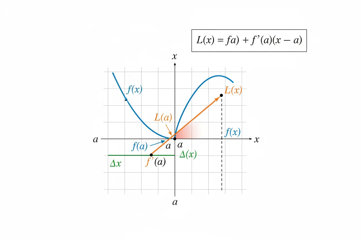
Linear approximation estimates a function near a known point by replacing the function locally with its tangent line. If f is differentiable at x = a, its linear approximation is L(x) = f(a) + f′(a)(x − a). The formula works because a differentiable curve becomes increasingly similar to its tangent line when viewed sufficiently close to the point of tangency. Linear approximation is especially useful for estimating roots, powers, trigonometric values, and other expressions near values that are easy to calculate exactly. It also gives a practical interpretation of the derivative: f′(a) converts a small input change into an approximate output change. In differential notation, the same idea is written Δy ≈ dy = f′(a)Δx. The estimate is generally strongest for small changes and may deteriorate as the evaluation point moves farther from a or the function has significant curvature. Linear approximation is therefore a local tool, not a claim that a nonlinear function is globally linear.
What Is Linear Approximation?
Suppose:
y = f(x)
and suppose f is differentiable at:
x = a
The tangent line at x = a has slope:
f′(a)
and passes through:
(a, f(a))
Using point-slope form:
y − f(a) = f′(a)(x − a)
Solve for y:
y = f(a) + f′(a)(x − a)
This tangent-line function is the linear approximation:
L(x) = f(a) + f′(a)(x − a)
For x near a:
f(x) ≈ L(x)
Linear Approximation Formula
The main formula is:
L(x) = f(a) + f′(a)(x − a)
where:
- a is the nearby reference point,
- f(a) is the known function value,
- f′(a) is the tangent slope,
- x − a is the input displacement,
- L(x) is the estimated function value.
Equivalently:
f(a + Δx) ≈ f(a) + f′(a)Δx
where:
Δx = x − a
This second form emphasizes small changes.
Why Linear Approximation Works
Differentiability means that sufficiently close to a point, the function’s change is dominated by a linear term.
Conceptually:
f(a + Δx) = f(a) + f′(a)Δx + error
where the error becomes small relative to Δx as:
Δx → 0
This limiting behavior connects linear approximation with the broader theory of limits.
The tangent line is therefore not merely visually close to the curve. It is the function’s best first-order linear model near the point.
How to Find a Linear Approximation
To find the linear approximation of f near x = a:
- Calculate f(a).
- Find the derivative f′(x).
- Evaluate f′(a).
- Substitute into:
L(x) = f(a) + f′(a)(x − a)
- Use L(x) to estimate f(x) for nearby x.
The reference point should ideally have an easy exact function value and be close to the value you want to estimate.
Basic Example
Find the linear approximation of:
f(x) = x²
near:
a = 3
First:
f(3) = 9
The derivative is:
f′(x) = 2x
So:
f′(3) = 6
Therefore:
L(x) = 9 + 6(x − 3)
Simplify:
L(x) = 6x − 9
Near x = 3:
x² ≈ 6x − 9
For example, at x = 3.01:
L(3.01) = 9 + 6(0.01)
= 9.06
The exact value is:
3.01² = 9.0601
The approximation is very close.
Estimate a Square Root
Estimate:
√25.4
Use:
f(x) = √x
Choose the nearby easy point:
a = 25
Then:
f(25) = 5
The derivative is:
f′(x) = 1/(2√x)
So:
f′(25) = 1/10
The linear approximation is:
L(x) = 5 + (1/10)(x − 25)
At:
x = 25.4
we obtain:
L(25.4) = 5 + (1/10)(0.4)
= 5.04
Therefore:
√25.4 ≈ 5.04
The actual value is approximately:
5.03984
so the estimate is close.
Estimate a Cube Root
Estimate:
∛8.12
Let:
f(x) = ∛x = x¹ᐟ³
Choose:
a = 8
Then:
f(8) = 2
Differentiate:
f′(x) = 1/(3x²ᐟ³)
At x = 8:
8²ᐟ³ = 4
so:
f′(8) = 1/12
Therefore:
L(x) = 2 + (1/12)(x − 8)
At x = 8.12:
L(8.12) = 2 + 0.12/12
= 2.01
Thus:
∛8.12 ≈ 2.01
Estimate a Reciprocal
Estimate:
1/1.02
Let:
f(x) = 1/x
Choose:
a = 1
Then:
f(1) = 1
and:
f′(x) = −1/x²
so:
f′(1) = −1
The linear approximation is:
L(x) = 1 − (x − 1)
At:
x = 1.02
we get:
L(1.02) = 1 − 0.02
= 0.98
The exact value is approximately:
0.98039
Therefore:
1/1.02 ≈ 0.98
Estimate a Trigonometric Value
Estimate:
sin(0.03)
using a linear approximation near:
a = 0
Let:
f(x) = sin x
Then:
f(0) = 0
and:
f′(x) = cos x
so:
f′(0) = 1
Therefore:
L(x) = x
Near zero:
sin x ≈ x
when angles are measured in radians.
Thus:
sin(0.03) ≈ 0.03
This familiar approximation is a direct tangent-line result.
Approximation of cos x Near Zero
Let:
f(x) = cos x
At:
a = 0
we have:
f(0) = 1
and:
f′(x) = −sin x
so:
f′(0) = 0
Therefore:
L(x) = 1
The first-order approximation is:
cos x ≈ 1
near x = 0.
Because the tangent line is horizontal there, first-order linear approximation does not capture the leading curvature term.
This explains why some functions require a higher-order approximation for substantially better precision.
Linear Approximation and the Derivative
The derivative f′(a) measures the instantaneous rate at which the output changes with the input.
For a small change:
Δx
the corresponding output change is approximately:
Δy ≈ f′(a)Δx
Therefore:
f(a + Δx) ≈ f(a) + f′(a)Δx
The derivative is not merely a tangent slope; it is the coefficient in the best local first-order approximation.
Linear Approximation and Differentials
The same approximation can be written using differentials.
Let:
dx = Δx
Then:
dy = f′(a)dx
and:
Δy ≈ dy
Therefore:
f(a + dx) ≈ f(a) + dy
For example, with:
f(x) = x²
at:
x = 3
and:
dx = 0.02
we get:
dy = 2(3)(0.02)
= 0.12
So:
f(3.02) ≈ 9 + 0.12
= 9.12
The exact value is:
9.1204
Actual Change Versus Linearized Change
The actual output change is:
Δy = f(a + Δx) − f(a)
The linearized change is:
dy = f′(a)Δx
Generally:
Δy ≠ dy
but for small Δx:
Δy ≈ dy
For:
f(x) = x²
we can calculate exactly:
Δy = (a + Δx)² − a²
= 2aΔx + (Δx)²
while:
dy = 2aΔx
Therefore:
Δy − dy = (Δx)²
The omitted term is quadratic, which becomes much smaller than Δx near zero.
Error in Linear Approximation
Define the approximation error:
E(x) = f(x) − L(x)
At the reference point:
E(a) = 0
Also, because L has the same derivative as f at a:
E′(a) = 0
Thus the approximation matches both the function value and slope at the reference point.
For smooth nonlinear functions, curvature determines how rapidly the error grows away from a.
The exact error analysis belongs to higher-order approximation methods, but the practical rule is simple: stay close to the reference point.
Choosing the Reference Point
A good reference point a should satisfy two conditions.
It should be close to the target x-value.
It should also make:
f(a)
and:
f′(a)
easy to calculate.
For estimating:
√15.8
a convenient reference is:
a = 16
rather than a more distant perfect square such as 9.
The closeness generally improves the approximation.
Example: Estimate √15.8
Let:
f(x) = √x
and choose:
a = 16
Then:
f(16) = 4
and:
f′(16) = 1/(2·4)
= 1/8
Therefore:
L(x) = 4 + (1/8)(x − 16)
At:
x = 15.8
we have:
x − 16 = −0.2
So:
L(15.8) = 4 − 0.2/8
= 4 − 0.025
= 3.975
Therefore:
√15.8 ≈ 3.975
The negative change is consistent with 15.8 being slightly below 16.
Overestimation and Underestimation
Whether a tangent-line approximation lies above or below the actual function depends on curvature.
If the function is concave up near a, its graph typically lies above its tangent line locally, so the linear approximation tends to underestimate.
If the function is concave down, the tangent line tends to lie above the graph, producing an overestimate.
For example:
f(x) = √x
is concave down for x > 0.
Therefore its tangent-line approximation near a positive point typically overestimates nearby square roots.
Our estimate:
√25.4 ≈ 5.04
is slightly above the actual value:
5.03984
which is consistent with this geometry.
Linear Approximation of eˣ Near Zero
Let:
f(x) = eˣ
At:
a = 0
we have:
f(0) = 1
and:
f′(0) = 1
Therefore:
L(x) = 1 + x
So near zero:
eˣ ≈ 1 + x
For example:
e^0.02 ≈ 1.02
The actual value is approximately:
1.02020
This is another widely used first-order approximation.
Linear Approximation of ln x Near 1
Let:
f(x) = ln x
Choose:
a = 1
Then:
f(1) = 0
and:
f′(x) = 1/x
so:
f′(1) = 1
Therefore:
L(x) = x − 1
Near x = 1:
ln x ≈ x − 1
For example:
ln(1.03) ≈ 0.03
The actual value is approximately:
0.02956
Linearization
The word linearization often refers to the specific linear function:
L(x) = f(a) + f′(a)(x − a)
Linear approximation refers to using that linearization to estimate f(x).
In practice, the terms are often used closely together.
The key object is the tangent-line model centered at the chosen reference point.
Linear Approximation From a Known Point and Slope
Sometimes the function formula is less important than the known data.
Suppose:
f(10) = 25
and:
f′(10) = 3
Then the linear approximation near x = 10 is:
L(x) = 25 + 3(x − 10)
To estimate:
f(10.2)
calculate:
L(10.2) = 25 + 3(0.2)
= 25.6
No explicit formula for f is required.
Linear Approximation and Tangent Lines
The approximation is literally the tangent line.
For:
y = f(x)
at:
x = a
the tangent-line equation is:
y − f(a) = f′(a)(x − a)
Therefore:
y = f(a) + f′(a)(x − a)
which is exactly:
L(x)
The geometric tangent and the numerical approximation are two interpretations of the same formula.
Linear Approximation and Limits
The underlying reason tangent lines approximate smooth curves is expressed through a limit.
Differentiability at a can be characterized by:
f(a + h) = f(a) + f′(a)h + r(h)
where the remainder satisfies:
r(h)/h → 0 as h → 0
This means the error becomes negligible compared with the first-order displacement h.
Thus the tangent-line approximation is justified by a precise limiting relationship.
Linear Approximation and Continuity
Differentiability implies continuity at the reference point.
If a function has a jump or other serious discontinuity at a, there cannot be an ordinary tangent-line linearization there.
Continuity alone, however, is not enough.
For example:
f(x) = |x|
is continuous at zero but has no unique derivative there because the left and right slopes differ.
Therefore it has no ordinary single linear approximation at x = 0 in the differentiability sense used here.
Linear Approximation and Implicit Differentiation
A function need not be explicitly solved for y before a tangent-line approximation can be built.
For an implicit curve, implicit differentiation can supply:
dy/dx
at the point.
Suppose:
x² + y² = 25
At:
(3, 4)
implicit differentiation gives:
dy/dx = −x/y
so:
dy/dx = −3/4
The local linear relation is:
y − 4 ≈ (−3/4)(x − 3)
This approximates the circle locally near (3, 4).
Multivariable Linear Approximation
For:
z = f(x, y)
the idea extends to:
f(a + Δx, b + Δy)
≈ f(a, b) + fₓ(a, b)Δx + fᵧ(a, b)Δy
Using the gradient:
∇f(a, b) = (fₓ(a, b), fᵧ(a, b))
we can write:
f(a + Δx, b + Δy)
≈ f(a, b) + ∇f(a, b) · (Δx, Δy)
This is the local tangent-plane approximation used in multivariable calculus.
Multivariable Example
Let:
f(x, y) = x² + xy + y²
Approximate the change near:
(2, 1)
when:
Δx = 0.01
and:
Δy = −0.02
First calculate:
fₓ = 2x + y
fᵧ = x + 2y
At (2, 1):
fₓ = 5
fᵧ = 4
Therefore:
Δf ≈ 5(0.01) + 4(−0.02)
= 0.05 − 0.08
= −0.03
The function is predicted to decrease by approximately 0.03.
Directional Interpretation
If a small multivariable displacement is:
Δr = uΔs
where u is a unit vector, then:
Δf ≈ ∇f · u Δs
But:
∇f · u
is the directional derivative.
Therefore:
Δf ≈ Dᵤf Δs
This shows that directional derivatives provide the linear rate used to estimate change along a chosen direction.
Linear Approximation and Related Rates
A related rates problem uses derivatives to connect changing quantities over time.
Linear approximation uses essentially the same local relationship over a small finite change.
If:
y = f(x)
then:
dy = f′(x)dx
For rates:
dy/dt = f′(x)dx/dt
For small changes:
Δy ≈ f′(x)Δx
The derivative is the shared local conversion factor.
Linear Approximation and Optimization
Local linear behavior is important in optimization because the gradient identifies the first-order direction of increase or decrease.
For one variable, if:
f′(a) > 0
the local linearization rises as x increases.
If:
f′(a) < 0
it falls.
If:
f′(a) = 0
the linear approximation becomes locally constant:
L(x) = f(a)
At such a critical point, first-order information alone cannot determine whether the point is a maximum, minimum, or neither.
Higher-order behavior becomes important.
Linear Approximation Versus Linear Transformation
A linear transformation is a linear algebra object satisfying properties such as:
T(u + v) = T(u) + T(v)
and:
T(cu) = cT(u)
A linear approximation is different.
It locally replaces a potentially nonlinear function by an affine expression:
L(x) = f(a) + f′(a)(x − a)
Because of the constant term, L is not necessarily a linear transformation in the strict linear-algebra sense.
The concepts both involve first-degree structure but serve different mathematical purposes.
Linear Approximation and Matrix Addition
In multivariable problems, derivative information can be represented using vectors and matrices, but matrix addition is an algebraic operation rather than an approximation method.
For example, the differential of a vector-valued function may involve adding first-order contributions from several variables.
The addition obeys ordinary vector or matrix rules, while linear approximation determines why only those first-order terms are retained locally.
Keeping these roles separate avoids confusing linear algebra operations with tangent-line approximation.
Linear Approximation and Line Integrals
A line integral accumulates values along a curve.
Linear approximation instead models a function in a small neighborhood of one point.
The concepts interact when a curve is divided into many small pieces: local derivative information can describe changes over each small displacement, while integration can accumulate effects over the full path.
For a gradient field:
dφ ≈ ∇φ · dr
and integrating those local changes along a path produces the net change in φ.
Linear Approximation and Integration by Substitution
Integration by substitution is an exact change-of-variable technique for suitable integrals.
Linear approximation does not change variables and generally produces an estimate rather than an exact identity away from the reference point.
The two ideas can appear in the same broader calculus problem, but their purposes are different.
Substitution simplifies integration structure; linear approximation simplifies local function behavior.
Linear Approximation and Error Propagation
Suppose a measured input x has a small possible error:
Δx
For:
y = f(x)
the resulting approximate error is:
Δy ≈ f′(x)Δx
In differential form:
dy = f′(x)dx
For example, if:
A = πr²
then:
dA = 2πr dr
If:
r = 10
and:
dr = 0.01
then:
dA = 2π(10)(0.01)
= 0.2π
≈ 0.628
So the area changes by approximately 0.628 square units for that small radius change.
Relative Error
For:
y = f(x)
an approximate relative output error is:
dy/y
For the circle area:
A = πr²
we have:
dA = 2πr dr
Divide by A:
dA/A = 2πr dr/(πr²)
= 2dr/r
Thus the relative area error is approximately twice the relative radius error.
If the radius has a small 1% measurement error, the area has an approximate 2% relative error.
This is a direct application of first-order linearization.
When Linear Approximation Is Exact
If the original function is already affine:
f(x) = mx + b
then:
f′(x) = m
and the tangent line at every point is the function itself.
Therefore:
L(x) = f(x)
exactly for all x.
The approximation error is zero because there is no curvature.
For nonlinear functions, the equality generally holds only at the reference point, with approximation nearby.
Why Distance From a Matters
Linear approximation is local.
Suppose:
f(x) = x²
near:
a = 1
Then:
L(x) = 1 + 2(x − 1)
= 2x − 1
At:
x = 1.01
the estimate is excellent.
At:
x = 10
the estimate is:
19
while:
f(10) = 100
The tangent line has not changed, but the quadratic curve has moved far away from it.
This demonstrates why the phrase “near a” is essential.
Curvature and Approximation Quality
Two functions can have the same value and slope at a point but diverge differently away from that point because their curvature differs.
Linear approximation ignores second-order and higher-order behavior.
Functions with strong curvature can therefore accumulate noticeable errors even for moderately small displacements.
The first derivative determines the tangent line, while higher derivatives influence how rapidly the curve separates from that line.
Linear Approximation Near a Critical Point
Suppose:
f′(a) = 0
Then:
L(x) = f(a)
The first-order approximation is constant.
For:
f(x) = x²
near:
a = 0
we have:
L(x) = 0
This correctly captures the zero slope but not the quadratic growth away from zero.
Thus first-order approximation may be relatively weak near stationary points when the second-order term dominates the change.
Approximation With Negative Δx
The method works on either side of a as long as the target remains sufficiently close and within the domain.
Suppose:
f(x) = √x
near:
a = 100
Then:
f(100) = 10
and:
f′(100) = 1/20
Estimate:
√99
Here:
Δx = −1
So:
√99 ≈ 10 + (1/20)(−1)
= 9.95
The actual value is approximately:
9.94987
The sign of Δx naturally moves the estimate downward.
Domain Restrictions
A tangent-line formula should be centered at a point where the function is differentiable.
For:
f(x) = √x
the ordinary derivative:
1/(2√x)
is not defined at:
x = 0
so the usual finite-slope linearization does not apply there.
For logarithms, the reference point must lie in the positive real domain.
For rational functions, denominator zeros must be avoided.
Domain checks are therefore part of choosing a valid reference point.
Linear Approximation and Local Units
Suppose f measures dollars and x measures units produced.
Then:
f′(a)
has units:
dollars per unit
Multiplying by:
Δx
gives:
dollars
So:
f′(a)Δx
has the same units as the change in f.
This unit consistency helps interpret linear approximations in physical and applied settings.
Common Mistakes With Linear Approximation
A common mistake is using:
f′(x)
instead of evaluating the derivative at the reference point:
f′(a)
The linearization must have a fixed slope.
Another error is forgetting the displacement:
x − a
and writing:
f(a) + f′(a)x
which generally gives the wrong tangent line.
The reference point should be close to the target and chosen so that the necessary values are known.
Students may also report the differential dy as though it were always exactly equal to the actual change Δy. In nonlinear problems:
Δy ≈ dy
rather than:
Δy = dy
Another mistake is using linear approximation far from the reference point without checking whether the error has become significant.
Finally, a zero derivative does not mean the function itself is locally constant; it only means its first-order linear term vanishes.
Frequently Asked Questions
What is linear approximation?
Linear approximation replaces a differentiable function near a point with its tangent-line function to estimate nearby values.
What is the linear approximation formula?
At x = a:
L(x) = f(a) + f′(a)(x − a)
Why does linear approximation work?
Differentiability means the function’s first-order local behavior is captured by its tangent line, with the remaining error becoming small relative to the displacement as x approaches a.
Is linear approximation the same as a tangent line?
The linearization L(x) is exactly the tangent-line function. Linear approximation refers to using that line to estimate nearby values of f.
How do you choose a reference point?
Choose a point close to the target where f(a) and f′(a) are easy to calculate exactly.
What is the differential form of linear approximation?
For small Δx:
Δy ≈ dy = f′(a)Δx
Does linear approximation give an exact answer?
It is exact for affine functions. For nonlinear functions, it is generally an approximation except at the reference point itself.
Why does the estimate get worse farther from a?
The tangent line captures only first-order local behavior. Curvature and higher-order effects become more important as the distance from the reference point increases.
Can linear approximation be used in several variables?
Yes. For f(x, y):
Δf ≈ fₓΔx + fᵧΔy
or:
Δf ≈ ∇f · Δr
What happens if f′(a) = 0?
The first-order approximation is:
L(x) = f(a)
Higher-order behavior may then be especially important.
How can you tell whether a tangent approximation overestimates or underestimates?
Local concavity provides a useful guide. A concave-up graph generally lies above its tangent line, while a concave-down graph generally lies below it near the point.
How do you check a linear approximation?
Verify f(a), f′(a), and the displacement x − a. Then compare with an exact or calculator value when available to judge the size and direction of the approximation error.




