

Confidence Intervals: Definition, Formula & Example

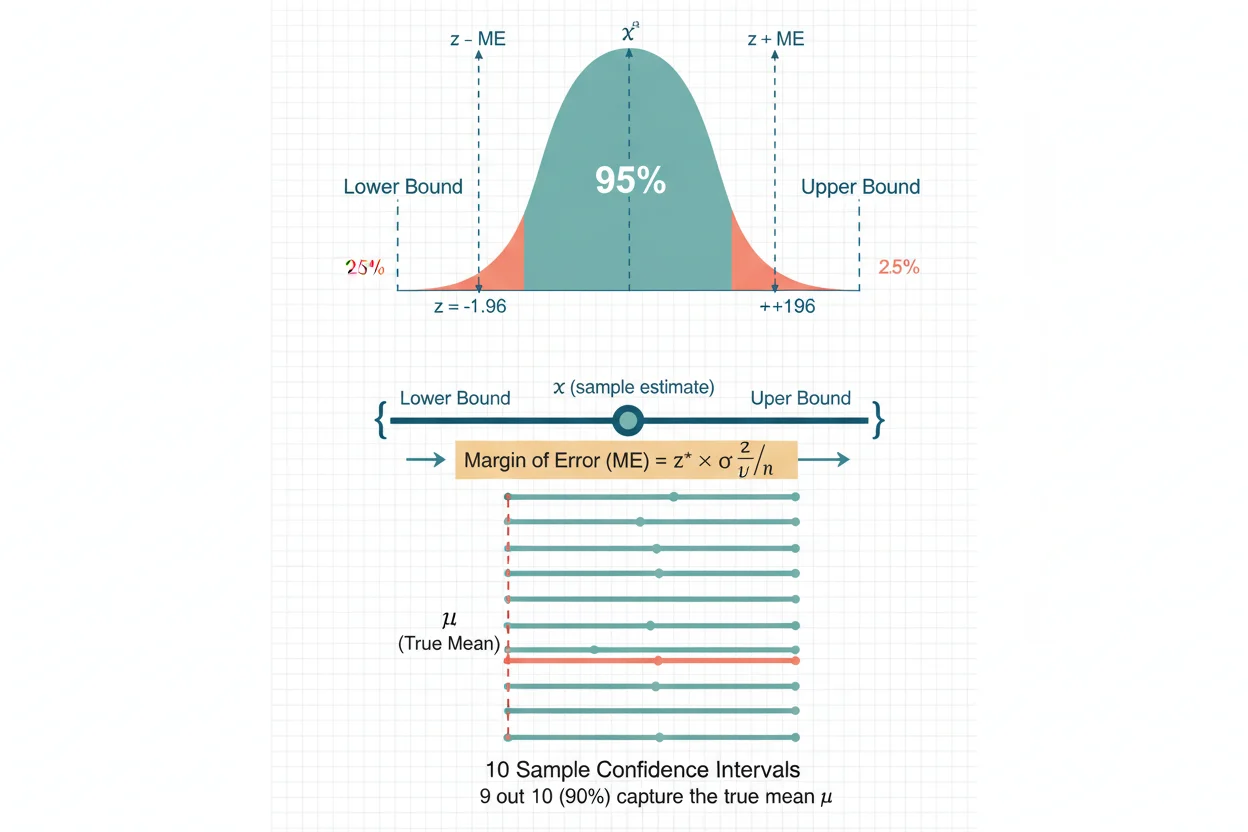
Confidence intervals estimate an unknown population parameter by giving a range of plausible values rather than only a single point estimate. A sample mean, proportion, difference, or other statistic provides the center of an interval, while its standard error and an appropriate critical value determine how far the interval extends on either side. A narrower confidence interval represents greater statistical precision under the assumptions of the procedure, whereas a wider interval represents greater uncertainty. The familiar 95% confidence interval comes from a repeated-sampling procedure designed so that approximately 95% of intervals constructed in the same way contain the fixed population parameter when the model assumptions hold. It does not mean there is a 95% frequentist probability that the parameter lies inside an interval that has already been calculated. Confidence intervals also provide more information than a bare significance decision because they show the estimated effect, its uncertainty, and which parameter values remain compatible with the data. Their validity depends on choosing the correct standard error, reference distribution, assumptions, and sampling procedure.
Confidence intervals are a central part of statistical inference within core statistics and the broader Statistics & Probability framework. Their construction is closely connected with sampling distributions, while the separate concept of confidence level determines the long-run coverage target used by the procedure.
What Are Confidence Intervals?
A confidence interval is an interval estimate for an unknown population parameter.
Instead of reporting only:
Estimate = 72
an analysis might report:
95% confidence interval = (67.94, 76.06)
The interval communicates both the point estimate and the uncertainty associated with estimating a population quantity from a sample.
The general structure is:
Confidence interval = point estimate ± margin of error
and:
Margin of error = critical value × standard error
Therefore:
Confidence interval = point estimate ± critical value × standard error
This framework appears repeatedly throughout inferential statistics.
The exact point estimate, standard error, and critical value depend on what parameter is being estimated and what assumptions are appropriate.
General Confidence Interval Formula
A large class of confidence intervals can be represented as:
Estimate ± critical value × SE(estimate)
where:
- Estimate = sample statistic used to estimate the population parameter
- SE = standard error of that statistic
- critical value = value determined by the reference distribution and confidence level
The lower confidence limit is:
Lower bound = Estimate − critical value × SE
The upper confidence limit is:
Upper bound = Estimate + critical value × SE
The quantity:
critical value × SE
is the margin of error.
For example, if:
Estimate = 50
and:
Margin of error = 4
then:
Lower bound = 50 − 4 = 46
Upper bound = 50 + 4 = 54
so the confidence interval is:
(46, 54)
Not every confidence interval is symmetric around its estimate, but the estimate ± margin-of-error form covers many commonly taught intervals.
What Does a 95% Confidence Interval Mean?
The correct frequentist interpretation concerns the procedure, not a probability assigned to the fixed parameter after observing the sample.
Imagine repeatedly:
- drawing a sample using the same sampling process,
- calculating an interval using the same formula,
- repeating this process many times.
If the procedure has 95% coverage and its assumptions hold, approximately 95% of those intervals would contain the true population parameter in the long run.
Some intervals would miss it.
For one already-computed frequentist interval, the population parameter is treated as fixed. The interval either contains that parameter or it does not.
Therefore, the statement:
“There is a 95% probability that this particular interval contains μ.”
is not the standard frequentist interpretation.
A more appropriate statement is:
“This interval was produced by a procedure with 95% long-run coverage under the model assumptions.”
In ordinary applied communication, analysts often say they are “95% confident” that the parameter lies within the interval, but that wording should be understood through the repeated-sampling interpretation.
Confidence Level
The confidence level represents the long-run coverage target of a confidence interval procedure.
Common choices include:
90%
95%
99%
If the confidence level is:
1 − α
then:
α = 1 − confidence level
For a 95% confidence interval:
α = 1 − 0.95 = 0.05
For a two-sided interval, the omitted probability is typically divided between the two tails:
α/2 = 0.025
The deeper interpretation and comparison of these levels belongs with confidence level, while the important point for constructing confidence intervals is that a higher coverage target generally requires a larger critical value and therefore a wider interval, all else equal.
Point Estimate
A confidence interval begins with a point estimate.
For a population mean μ, the usual point estimate is the sample mean:
x̄
For a population proportion p, the sample proportion is:
p̂ = x/n
where x is the number of successes and n is the sample size.
For a difference between two population means, the point estimate is commonly:
x̄₁ − x̄₂
The point estimate identifies the center of many confidence intervals, but by itself it does not quantify sampling uncertainty.
Two studies can produce the same estimate while having dramatically different levels of precision because their sample sizes or sample variability differ.
Standard Error
The standard error measures how much a sample statistic would typically vary across repeated samples under the assumed model.
For a sample mean when the population standard deviation σ is known:
SE(x̄) = σ/√n
When σ is unknown and the sample standard deviation s is used:
Estimated SE(x̄) = s/√n
For a sample proportion:
SE(p̂) ≈ √[p̂(1 − p̂)/n]
under the usual large-sample approximation.
A smaller standard error generally produces a narrower confidence interval.
The standard error is not the same as the standard deviation of the raw observations. The standard deviation describes variability among individual observations, whereas the standard error describes sampling variability of an estimator.
Margin of Error
The margin of error is:
ME = critical value × SE
If the confidence interval has the symmetric form:
Estimate ± ME
then its total width is:
Width = 2 × ME
Suppose:
critical value = 1.96
and:
SE = 3
Then:
ME = 1.96 × 3
ME = 5.88
If the estimate is 50:
CI = 50 ± 5.88
so:
Lower bound = 44.12
Upper bound = 55.88
The resulting confidence interval is:
(44.12, 55.88)
Confidence Interval for a Population Mean When σ Is Known
If a population standard deviation σ is known and the relevant normal-theory conditions are satisfied, a confidence interval for the population mean μ is:
x̄ ± z*σ/√n
where:
- x̄ = sample mean
- σ = population standard deviation
- n = sample size
- z* = critical value from the standard normal distribution
For a conventional two-sided 95% confidence interval:
z* ≈ 1.96
Therefore:
95% CI = x̄ ± 1.96σ/√n
In practice, knowing the true population standard deviation is relatively uncommon, so t-based intervals are frequently more relevant for means.
Confidence Interval for a Population Mean When σ Is Unknown
When σ is unknown, it is commonly estimated using the sample standard deviation s.
The confidence interval becomes:
x̄ ± t*s/√n
where t* is an appropriate critical value from a t distribution.
For a one-sample mean:
df = n − 1
The use of a t critical value accounts for additional uncertainty created by estimating σ with s.
As the degrees of freedom increase, the t distribution approaches the standard normal distribution, so t critical values approach corresponding z critical values.
Confidence Interval Example for a Mean
Suppose a random sample contains:
n = 36
observations.
The sample mean is:
x̄ = 72
and the sample standard deviation is:
s = 12
We want a 95% confidence interval for the population mean μ.
Because the population standard deviation is unknown, use a t interval.
Step 1: Calculate the Standard Error
SE = s/√n
SE = 12/√36
SE = 12/6
SE = 2
Step 2: Determine Degrees of Freedom
df = n − 1
df = 36 − 1
df = 35
For a two-sided 95% confidence interval with 35 degrees of freedom:
t* ≈ 2.030
Step 3: Calculate the Margin of Error
ME = t* × SE
ME ≈ 2.030 × 2
ME ≈ 4.06
Step 4: Calculate the Bounds
Lower bound = 72 − 4.06
Lower bound = 67.94
and:
Upper bound = 72 + 4.06
Upper bound = 76.06
Therefore:
95% CI ≈ (67.94, 76.06)
The estimate of the population mean is 72, with a 95% confidence interval extending from approximately 67.94 to 76.06 under the assumptions of the t procedure.
How to Interpret the Example
The correct interpretation is not that the probability of μ lying between 67.94 and 76.06 is now exactly 95% under the frequentist model.
Instead, the interval was constructed using a method that would capture μ approximately 95% of the time over repeated samples when its assumptions are satisfied.
The interval also communicates precision.
An interval from:
67.94 to 76.06
is more informative than merely reporting:
x̄ = 72
because it shows how uncertain that estimate is.
Why a t Critical Value Is Larger Than a z Critical Value
When σ is estimated from sample data, there is additional uncertainty.
The t distribution accounts for this through heavier tails.
For a 95% interval:
z* ≈ 1.96
but with 35 degrees of freedom:
t* ≈ 2.030
With very small degrees of freedom, the difference is larger.
As the sample size grows:
df = n − 1
also grows, and:
t* → z*
for corresponding confidence levels.
This is why t-based and z-based intervals become increasingly similar in large samples.
Confidence Interval for a Population Proportion
Suppose x successes are observed among n binary trials or observations.
The sample proportion is:
p̂ = x/n
A commonly taught large-sample confidence interval is:
p̂ ± z*√[p̂(1 − p̂)/n]
The interval estimates an unknown population proportion p.
This form is often called the Wald interval.
It is mathematically simple, but it can perform poorly with small samples or when p̂ is close to 0 or 1. Methods such as the Wilson interval often have better coverage properties.
The binary sampling structure connects proportion estimation with the binomial distribution and calculations involving binomial probability, although estimating p is a different task from calculating the probability of a count when p is already specified.
Confidence Interval Example for a Proportion
Suppose 120 successes are observed among 200 independent observations.
Then:
p̂ = 120/200
p̂ = 0.60
For a 95% large-sample interval:
z* ≈ 1.96
The estimated standard error is:
SE ≈ √[(0.60)(0.40)/200]
SE ≈ √0.0012
SE ≈ 0.03464
The margin of error is:
ME ≈ 1.96 × 0.03464
ME ≈ 0.0679
Therefore:
Lower bound ≈ 0.60 − 0.0679 = 0.5321
Upper bound ≈ 0.60 + 0.0679 = 0.6679
The approximate confidence interval is:
95% CI ≈ (0.532, 0.668)
or approximately:
53.2% to 66.8%
This calculation uses the simple large-sample Wald formula. An analyst may choose a method with better finite-sample coverage when greater accuracy is required.
Confidence Intervals and Sample Size
Sample size has a major effect on interval precision.
For a mean:
SE = σ/√n
or approximately:
SE = s/√n
Increasing n therefore reduces the standard error at a rate proportional to:
1/√n
This has an important consequence.
To reduce the standard error by half, the sample size must generally be multiplied by four.
For example:
n = 100 → √n = 10
while:
n = 400 → √n = 20
The denominator doubles, so the standard error is approximately halved when the other quantities remain comparable.
Confidence intervals therefore become narrower as sample size increases, but precision improves with the square root of n rather than proportionally with n.
Confidence Intervals and Variability
Greater variability produces greater uncertainty.
For a mean:
SE = s/√n
If s increases while n remains constant, the standard error increases.
The confidence interval consequently becomes wider.
This makes intuitive sense. When observations vary substantially, the sample mean is generally a less precise indicator of the population mean than when observations are tightly concentrated.
Sample size and variability therefore work in opposite directions:
Larger n → narrower interval
Larger variability → wider interval
when other factors remain unchanged.
Confidence Intervals and Confidence Level
Increasing the confidence level generally increases interval width.
For the standard normal distribution, common two-sided critical values are approximately:
| Confidence Level | z* |
|---|---|
| 90% | 1.645 |
| 95% | 1.960 |
| 99% | 2.576 |
Suppose the estimate and standard error are unchanged.
A 99% confidence interval uses a larger critical value than a 95% confidence interval, so it extends farther from the point estimate.
This reflects a tradeoff:
Higher confidence → wider interval
Narrower interval → lower confidence, all else equal
Obtaining both substantially greater confidence and substantially greater precision usually requires more information, often through a larger sample.
Width of a Confidence Interval
For a symmetric confidence interval:
Estimate ± critical value × SE
the width is:
Width = 2 × critical value × SE
Therefore, interval width depends directly on:
- the confidence level,
- the standard error,
- sample size,
- data variability,
- the chosen inferential procedure.
A narrow confidence interval is usually evidence of greater statistical precision, but narrowness alone does not guarantee validity.
A very narrow interval based on biased sampling, violated assumptions, poor measurement, or an inappropriate model can be precisely wrong.
Confidence Intervals and Statistical Significance
For many standard two-sided hypothesis tests, there is a close relationship between confidence intervals and significance tests.
Suppose the hypotheses are:
H₀: θ = θ₀
H₁: θ ≠ θ₀
and the significance level is:
α = 0.05
Under corresponding procedures, if the 95% confidence interval excludes θ₀, the two-sided test typically rejects H₀ at the 5% level.
If the interval includes θ₀, the corresponding test generally does not reject H₀.
For example, when estimating a mean difference, the null value is often:
0
If a corresponding 95% confidence interval is:
(1.4, 6.8)
zero is excluded, which aligns with statistical significance at the corresponding two-sided α = 0.05 level.
If the interval is:
(−1.2, 5.7)
zero is included, so the corresponding test would generally not reject H₀.
This relationship requires matching the interval and hypothesis-test procedures correctly.
Confidence Intervals Provide More Than a p-Value
A significance test may reduce the analysis to:
Reject H₀
or:
Do not reject H₀
A confidence interval provides additional quantitative information.
It shows:
- the estimated parameter,
- the direction of the estimate,
- the approximate magnitude,
- uncertainty around the estimate,
- parameter values compatible with the procedure.
Suppose two studies both produce p < 0.05.
One might report:
Mean difference = 0.2
95% CI = (0.01, 0.39)
while another reports:
Mean difference = 8.0
95% CI = (5.0, 11.0)
Both may be statistically significant, yet their estimated magnitudes and practical implications are very different.
Confidence intervals make that distinction visible.
Statistical Significance vs Practical Significance
A confidence interval should be interpreted in substantive units whenever possible.
Suppose a treatment produces an estimated improvement of:
0.5 units
with:
95% CI = (0.2, 0.8)
The interval excludes zero, so a corresponding test may be statistically significant.
However, if an improvement smaller than 5 units is practically unimportant, the result may have little practical significance despite strong statistical evidence of a nonzero effect.
Conversely, a wide confidence interval may contain both important positive effects and no effect. In that case, the study may simply be too imprecise to distinguish among substantively different possibilities.
Statistical significance and practical importance therefore answer different questions.
Confidence Intervals and Null Values
The relevant null value depends on the parameter.
For a difference:
θ₀ = 0
often represents no difference.
For a ratio:
θ₀ = 1
often represents no multiplicative association.
For a population correlation:
ρ₀ = 0
represents no linear correlation.
This matters because interpreting whether a confidence interval contains zero is only appropriate when zero is actually the meaningful null value for that parameter.
For example, confidence intervals for a correlation coefficient can help describe uncertainty in the estimated strength and direction of linear association, but the interval must respect the statistical properties of correlation rather than automatically applying a generic mean formula.
Confidence Intervals for Differences Between Means
When comparing two independent population means, the parameter may be:
μ₁ − μ₂
with point estimate:
x̄₁ − x̄₂
A general interval structure is:
(x̄₁ − x̄₂) ± critical value × SE(x̄₁ − x̄₂)
The exact standard error and degrees of freedom depend on assumptions about the samples and population variances.
For independent samples without assuming equal population variances, Welch’s approach is commonly appropriate.
A confidence interval around the difference is often more informative than merely stating that two sample means are numerically different because it quantifies uncertainty in the estimated population difference.
Confidence Intervals for Paired Data
When observations are naturally paired, the analysis should preserve that pairing.
Examples include:
- before-and-after measurements on the same individuals,
- matched subjects,
- paired experimental units.
Define each pairwise difference as:
dᵢ = measurement 1 − measurement 2
Then calculate the sample mean and standard deviation of those differences:
d̄
and:
s_d
A t-based interval for the population mean difference can have the form:
d̄ ± t*s_d/√n
The important distinction is that n represents the number of pairs and the variability is measured among the pairwise differences.
Treating paired observations as two unrelated samples discards the dependence structure and can give an inappropriate standard error.
Confidence Intervals for Variance
Confidence intervals are not limited to means and proportions.
Under normal-population assumptions, an interval for the population variance σ² can be constructed using the chi-square distribution.
The calculation depends on:
(n − 1)s²/σ²
which has a chi-square distribution with:
df = n − 1
under the normal model.
This illustrates that different parameters require different reference distributions. The chi-square distribution can therefore appear in variance estimation as well as categorical hypothesis-testing contexts.
A z or t critical value should not simply be inserted into every confidence interval problem.
One-Sided Confidence Bounds
Not every confidence procedure needs both a lower and upper bound.
Sometimes the question concerns only whether a parameter is above or below a meaningful threshold.
A one-sided procedure may produce:
Lower confidence bound = L
with an interval conceptually extending to:
(L, ∞)
or:
Upper confidence bound = U
with:
(−∞, U)
The critical value differs from that of a two-sided interval with the same nominal confidence percentage because the relevant tail probability is allocated differently.
Therefore, a 95% one-sided bound is not constructed using exactly the same critical value as a 95% two-sided interval.
Assumptions Behind Confidence Intervals
There is no single universal set of assumptions for all confidence intervals.
The required assumptions depend on the parameter and procedure.
Important considerations commonly include:
Sampling or Assignment Mechanism
Probability-based sampling or a justified experimental design supports the inferential link between sample statistics and population parameters.
A very large convenience sample can still produce biased estimates if it systematically excludes important parts of the target population.
Independence
Many standard formulas assume observations are independent.
Repeated observations, clusters, matched units, or time-dependent measurements may require specialized standard errors or models.
Distributional Conditions
Small-sample t procedures for means rely more strongly on assumptions concerning the distribution of errors or observations.
Large-sample procedures may be more robust in some settings because sampling distributions approach approximate limiting forms.
However, large samples do not automatically solve bias, dependence, or poor measurement.
Correct Standard Error
A confidence interval is only as trustworthy as its uncertainty estimate.
Using a standard error formula that assumes independence on highly clustered data can make the interval much too narrow.
Appropriate Reference Distribution
The interval may require a:
- z distribution,
- t distribution,
- chi-square distribution,
- F distribution,
- bootstrap distribution,
- exact discrete procedure,
- another model-specific distribution.
The method should follow the statistical problem rather than the convenience of a familiar formula.
Normality and Confidence Intervals
A common misconception is that all raw data must be perfectly normally distributed before a confidence interval can be calculated.
For a small-sample classical t interval for a mean, strong skewness or extreme outliers can be important because the sampling distribution may not be well approximated by the t model.
As sample size increases under suitable conditions, the sampling distribution of the sample mean often becomes more nearly normal even when the individual observations are not normal.
However, this robustness should not be overstated.
Severe outliers, dependence, extremely heavy tails, selection bias, or a poorly defined population can still undermine inference.
The appropriate diagnostic questions depend on the estimator and procedure being used.
Confidence Intervals and Outliers
Outliers can influence confidence intervals in several ways.
For a mean-based interval, an extreme observation can change:
x̄
and also increase:
s
The point estimate may therefore shift while the standard error becomes larger.
This can move and widen the confidence interval simultaneously.
Outliers should not automatically be deleted merely because they affect statistical results. Their origin should be investigated.
An outlier may represent:
- a data-entry error,
- a measurement problem,
- a genuine rare observation,
- an indication that the assumed model is inappropriate.
Statistical decisions should reflect the reason for the observation rather than a desire to obtain a narrower interval.
Confidence Intervals and Biased Samples
A confidence interval quantifies sampling uncertainty under a particular inferential procedure. It does not automatically correct systematic bias.
Suppose a survey estimates a population proportion using a very large but badly selected sample.
The resulting standard error may be tiny, producing a narrow confidence interval.
Yet if the sample systematically underrepresents part of the population, the interval may be centered around a biased estimate.
Therefore:
Narrow interval ≠ accurate estimate
Precision and bias are distinct statistical properties.
Confidence Intervals and Association
Confidence intervals can quantify uncertainty around measures of association, including correlation coefficients, regression coefficients, risk differences, ratios, and other parameters.
However, an interval that excludes a null association does not establish causation.
For example, an interval around a correlation may indicate evidence that the population linear correlation differs from zero. It does not show that changing one variable would cause a change in the other.
Study design, confounding, temporal ordering, measurement quality, and substantive knowledge remain necessary for causal conclusions.
Confidence Intervals From Binomial Data
When data consist of x successes out of n trials, the uncertainty around the population proportion can be handled using procedures based on the binomial model.
The simple normal approximation:
p̂ ± z*√[p̂(1 − p̂)/n]
is widely taught, but it is not always the best choice.
It can behave poorly when:
- n is small,
- the success count is near zero,
- the failure count is near zero.
More reliable methods can include Wilson, Agresti-Coull, or exact procedures depending on the inferential objective.
The underlying binomial probability model helps explain why proportion intervals behave differently near the boundaries 0 and 1.
Why Confidence Intervals Can Extend Beyond Logical Bounds
Some approximate formulas can produce impossible-looking endpoints.
For a proportion, the parameter must satisfy:
0 ≤ p ≤ 1
Yet a simple Wald interval can sometimes produce:
Lower bound < 0
or:
Upper bound > 1
particularly with small samples or proportions near 0 or 1.
That behavior is a warning about the approximation rather than evidence that probabilities can genuinely fall outside the 0-to-1 range.
Alternative interval procedures can respect the parameter boundaries more naturally.
Confidence Interval vs Prediction Interval
A confidence interval estimates uncertainty about a population parameter or mean response.
A prediction interval addresses uncertainty about a future individual observation.
Prediction intervals are generally wider because they must account for both:
- uncertainty in estimating the mean response, and
- natural variation among individual observations.
For example, an interval estimating the population mean height may be relatively narrow, while an interval predicting the height of a randomly selected future individual would be substantially wider.
Confusing these two intervals can lead to severe underestimation of predictive uncertainty.
Confidence Interval vs Tolerance Interval
A tolerance interval answers another distinct question.
A confidence interval may estimate a population mean.
A tolerance interval aims to contain a specified proportion of the population with a stated level of confidence.
These are not interchangeable.
For example, a narrow confidence interval for the mean does not imply that most individual observations lie within that interval.
The population itself can have substantial variation even when its mean is estimated very precisely.
Confidence Interval vs Credible Interval
A frequentist confidence interval and a Bayesian credible interval can sometimes have similar numerical endpoints but have different interpretations.
A Bayesian credible interval is constructed from a posterior probability distribution, which can be obtained through methods involving Bayes’ theorem and a specified prior and likelihood.
A 95% Bayesian credible interval can, under that model, be interpreted as containing 95% of the posterior probability for the parameter.
A classical 95% confidence interval instead describes the long-run coverage of a repeated-sampling procedure.
The distinction is conceptual, not merely terminological.
What Makes Confidence Intervals Narrower?
Holding other factors constant, confidence intervals tend to become narrower when:
- sample size increases,
- population or sample variability decreases,
- the chosen confidence level decreases,
- the estimator becomes more statistically efficient,
- study design provides more informative data.
However, reducing interval width should not be pursued by sacrificing validity.
For example, pretending correlated observations are independent may produce a smaller standard error and narrower interval, but the apparent precision would be misleading.
What Makes Confidence Intervals Wider?
Confidence intervals generally widen when:
- the confidence level increases,
- variability increases,
- sample size decreases,
- the standard error increases,
- a heavier-tailed reference distribution is required,
- the design contains less independent information.
A wide interval is not necessarily a statistical failure.
It may accurately reveal that the available data do not support a precise estimate.
Reporting that uncertainty is more informative than concealing it behind an overly precise point estimate.
Common Confidence Interval Mistakes
One of the most common mistakes is saying that a classical 95% confidence interval has a 95% probability of containing the fixed parameter after the interval has already been observed.
Another is confusing the confidence level with the percentage of sample observations contained inside the interval. A confidence interval for a mean is not intended to contain 95% of individual data points.
A third mistake is using a z critical value automatically when the appropriate procedure requires a t distribution or another reference distribution.
Analysts also sometimes confuse standard deviation with standard error. Standard deviation describes variability among observations; standard error describes uncertainty in an estimator.
Another error is concluding that overlapping confidence intervals necessarily imply no statistically significant difference, or that non-overlapping intervals provide a complete hypothesis test. The relationship depends on the exact parameters, dependence structure, and interval procedures.
It is also incorrect to equate statistical significance with practical importance.
Finally, confidence intervals cannot compensate for biased samples, severe model misspecification, invalid independence assumptions, or poor data quality.
How to Calculate Confidence Intervals Step by Step
A reliable general process is:
Step 1: Identify the Parameter
Determine whether the target is a:
- population mean,
- proportion,
- difference,
- variance,
- correlation,
- regression coefficient,
- another parameter.
Step 2: Choose the Point Estimate
For example:
μ → x̄
or:
p → p̂
Step 3: Determine the Standard Error
Use the standard error formula appropriate for the estimator and study design.
Step 4: Select the Confidence Level
For example:
95%
which corresponds to:
α = 0.05
for the usual two-sided setup.
Step 5: Choose the Reference Distribution
Depending on the problem, this might involve z, t, chi-square, or another distribution.
Step 6: Determine the Critical Value
For a standard two-sided 95% normal-based interval:
z* ≈ 1.96
For a t interval, the critical value additionally depends on the degrees of freedom.
Step 7: Calculate the Margin of Error
ME = critical value × SE
Step 8: Calculate the Interval Bounds
Lower = Estimate − ME
Upper = Estimate + ME
when a symmetric interval is appropriate.
Step 9: Interpret the Parameter and Uncertainty
Describe what parameter is being estimated, the interval endpoints, and the relevant assumptions without assigning an unsupported posterior probability to the fixed parameter.
How to Report Confidence Intervals
A useful statistical statement includes the point estimate and interval.
For example:
Mean = 72, 95% CI (67.94, 76.06)
or:
Estimated proportion = 0.60, 95% CI approximately (0.532, 0.668)
When relevant, the report should also make clear:
- what population parameter is being estimated,
- what interval procedure was used,
- whether important assumptions were required,
- what units the estimate uses.
Reporting an interval without identifying the parameter can make a technically correct calculation difficult to interpret.
Frequently Asked Questions About Confidence Intervals
What are confidence intervals?
Confidence intervals are ranges calculated from sample data to estimate unknown population parameters while expressing sampling uncertainty.
What is the general confidence interval formula?
A common general form is:
Estimate ± critical value × standard error
The exact critical value and standard error depend on the parameter and statistical procedure.
What is a 95% confidence interval?
A 95% confidence interval is produced by a procedure designed to contain the true parameter approximately 95% of the time over repeated samples when the method’s assumptions hold.
Does a 95% confidence interval mean there is a 95% probability the true value is inside it?
Not under the standard frequentist interpretation after the interval has been calculated. The 95% refers to the long-run coverage rate of the procedure.
What is the margin of error?
The margin of error is commonly:
ME = critical value × standard error
It determines how far a symmetric confidence interval extends from its point estimate.
What is the difference between standard deviation and standard error?
Standard deviation measures variability among individual observations. Standard error measures sampling variability of an estimator such as a sample mean.
What is the 95% confidence interval formula for a mean when σ is known?
The normal-based formula is:
x̄ ± 1.96σ/√n
for a conventional two-sided 95% interval under the required assumptions.
What if the population standard deviation is unknown?
For a mean, a t-based interval is commonly used:
x̄ ± t*s/√n
with:
df = n − 1
for the standard one-sample procedure.
Why do confidence intervals become narrower with larger samples?
Many standard errors decrease approximately as:
1/√n
so increasing sample size reduces sampling uncertainty and therefore narrows the interval when other factors remain similar.
Does doubling the sample size cut the margin of error in half?
Not generally. Because standard error commonly scales with 1/√n, approximately quadrupling the sample size is required to halve the margin of error when other quantities remain constant.
Why does a 99% confidence interval tend to be wider than a 95% confidence interval?
A 99% interval requires a larger critical value to achieve greater long-run coverage. The larger critical value increases the margin of error.
Can a confidence interval be statistically significant?
A confidence interval itself is not usually described as “significant,” but it can correspond to a hypothesis-test decision. For example, if an appropriate 95% interval for a difference excludes zero, the corresponding two-sided test typically rejects a zero-difference null hypothesis at α = 0.05.
Does a narrow confidence interval mean the estimate is correct?
No. A narrow interval indicates precision under the statistical procedure. Bias, invalid sampling, measurement error, dependence, or incorrect model assumptions can still make a precise estimate inaccurate.
Is a confidence interval the same as a prediction interval?
No. A confidence interval typically estimates a population parameter or mean response, while a prediction interval covers uncertainty for a future individual observation and is usually wider.
Is a confidence interval the same as a Bayesian credible interval?
No. A frequentist confidence interval has a repeated-sampling coverage interpretation. A Bayesian credible interval is derived from a posterior distribution and permits probability statements about the parameter conditional on the specified model and prior.
Can confidence intervals be used for proportions?
Yes. A population proportion can be estimated using several interval procedures. The simple large-sample formula is:
p̂ ± z*√[p̂(1 − p̂)/n]
although methods such as the Wilson interval can provide better performance in some situations.
Can confidence intervals be used for variance?
Yes. Under suitable assumptions, confidence intervals for population variance can be constructed using a chi-square reference distribution.
What does it mean when a confidence interval is very wide?
A wide interval indicates substantial uncertainty about the parameter under the chosen method. Small sample size, high variability, a high confidence level, or a less informative study design can all contribute.
Do confidence intervals prove causation?
No. Confidence intervals quantify uncertainty around estimated parameters. Causal conclusions depend on study design, assumptions, confounding control, and substantive evidence beyond the interval itself.




