


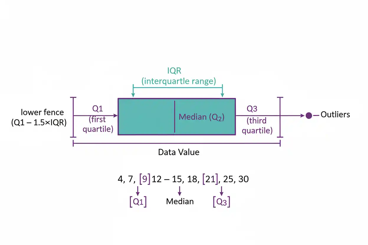
The interquartile range is a measure of statistical spread that describes the width of the middle 50% of an ordered data set. It is calculated by subtracting the first quartile Q₁ from the third quartile Q₃, giving the simple formula IQR = Q₃ − Q₁. Because the interquartile range depends on quartiles rather than the most extreme observations, it is considerably less sensitive to unusually large or small values than the ordinary range. This makes it especially useful for skewed distributions, data containing potential outliers, and descriptive summaries where a robust measure of variability is desirable. The interquartile range also forms the width of the box in a standard box plot and is commonly used to construct the 1.5 × IQR fences for identifying observations that warrant closer investigation. However, different statistical conventions can produce slightly different quartile values for the same finite sample, so the quartile method should be stated when exact numerical agreement matters. The interquartile range measures dispersion rather than center, probability, or causal relationships, and it should be interpreted alongside other features of the data rather than as a complete description by itself.
Within core statistics, the interquartile range provides a robust alternative to spread measures that depend heavily on every numerical value. It belongs to the broader Statistics & Probability framework alongside measures of center, probability models, regression methods, and statistical inference.
What Is the Interquartile Range?
The interquartile range measures the distance between the first and third quartiles.
Its formula is:
IQR = Q₃ − Q₁
where:
- Q₁ = first quartile, or lower quartile
- Q₃ = third quartile, or upper quartile
- IQR = interquartile range
Q₁ represents a location near the 25th percentile of the data.
Q₃ represents a location near the 75th percentile.
The interval from Q₁ to Q₃ therefore covers the central half of the ordered observations according to the chosen quartile convention.
The interquartile range is the width of that interval.
If:
Q₁ = 18
and:
Q₃ = 31
then:
IQR = 31 − 18
IQR = 13
The middle portion of the data spans 13 units.
Interquartile Range Formula
The interquartile range formula is:
IQR = Q₃ − Q₁
It is always nonnegative because:
Q₃ ≥ Q₁
for an ordered data set.
If:
Q₁ = Q₃
then:
IQR = 0
which means the first and third quartiles coincide.
This can happen when many observations have the same value.
Unlike variance, the interquartile range does not square deviations and does not use every observation directly. Its calculation depends only on the locations of Q₁ and Q₃.
What Are Quartiles?
Quartiles divide ordered data into four portions.
The three principal quartile locations are:
Q₁ = first quartile
Q₂ = second quartile
Q₃ = third quartile
Q₂ is the median.
Conceptually:
Q₁ ≈ 25th percentile
Q₂ ≈ 50th percentile
Q₃ ≈ 75th percentile
These statements describe the intended percentile locations, but the exact numerical quartile calculation for a finite sample depends on the convention being used.
Different textbooks, calculators, spreadsheets, and statistical packages can use different interpolation rules.
That difference does not mean one result is automatically wrong. It means the quartile definition must be identified when exact reproducibility matters.
How to Calculate the Interquartile Range
A common hand-calculation procedure is:
- Sort the observations from smallest to largest.
- Find the median.
- Find Q₁ as the median of the lower half.
- Find Q₃ as the median of the upper half.
- Calculate Q₃ − Q₁.
For an odd-sized data set, one common convention excludes the overall median when forming the lower and upper halves.
Other conventions exist, particularly in statistical software.
The important principle is to use one method consistently.
Interquartile Range Example With an Even Number of Values
Consider:
3, 5, 7, 8, 11, 13, 15, 18
The values are already ordered.
There are:
n = 8
observations.
Step 1: Find the Median
The middle two values are:
8 and 11
Therefore:
Median = (8 + 11)/2
Median = 9.5
Step 2: Find Q₁
The lower half is:
3, 5, 7, 8
Its median is:
Q₁ = (5 + 7)/2
Q₁ = 6
Step 3: Find Q₃
The upper half is:
11, 13, 15, 18
Its median is:
Q₃ = (13 + 15)/2
Q₃ = 14
Step 4: Calculate the Interquartile Range
IQR = Q₃ − Q₁
IQR = 14 − 6
IQR = 8
Therefore, the interquartile range is:
8
The middle 50% of the data spans from approximately 6 to 14 under this quartile convention.
Interquartile Range Example With an Odd Number of Values
Consider:
2, 4, 5, 7, 9, 10, 13, 16, 20
There are:
n = 9
observations.
The overall median is the fifth value:
Q₂ = 9
Using the common median-of-halves convention that excludes the overall median, the lower half is:
2, 4, 5, 7
and the upper half is:
10, 13, 16, 20
For the lower half:
Q₁ = (4 + 5)/2
Q₁ = 4.5
For the upper half:
Q₃ = (13 + 16)/2
Q₃ = 14.5
Therefore:
IQR = 14.5 − 4.5
IQR = 10
The interquartile range is:
10
Why Quartile Methods Can Give Different Answers
Suppose a calculator and textbook produce slightly different Q₁ or Q₃ values for the same data.
This often occurs because quartiles are not defined by one universally adopted finite-sample algorithm.
Possible methods include:
- medians of the lower and upper halves,
- inclusive quartile methods,
- exclusive quartile methods,
- percentile interpolation procedures.
For a large sample, these differences are usually relatively small.
For a small sample, they can be noticeable.
Therefore, when a problem specifies a particular quartile method or software package, use that method.
When calculating manually for instructional purposes, the median-of-halves convention is often used unless another method is stated.
Interquartile Range and the Five-Number Summary
The interquartile range is closely connected with the five-number summary:
Minimum
Q₁
Median
Q₃
Maximum
The five-number summary describes both center and spread while preserving information about the lower and upper portions of the distribution.
The interquartile range uses two of these values:
IQR = Q₃ − Q₁
The ordinary range instead uses:
Range = Maximum − Minimum
Because the range depends on the two most extreme values, it can change dramatically because of a single unusual observation.
The interquartile range is substantially more resistant.
Interquartile Range vs Range
Consider:
5, 6, 7, 8, 9, 10, 11, 12
The ordinary range is:
12 − 5 = 7
Now replace the maximum 12 with 100:
5, 6, 7, 8, 9, 10, 11, 100
The range becomes:
100 − 5 = 95
One observation changed the range from 7 to 95.
Under the median-of-halves method, the first data set has:
Q₁ = 6.5
Q₃ = 10.5
so:
IQR = 4
The modified data set also has:
Q₁ = 6.5
while:
Q₃ = (10 + 11)/2 = 10.5
so:
IQR = 4
The extreme value dramatically changes the range but does not change the interquartile range in this example.
This illustrates its robustness.
Why the Interquartile Range Is Robust
The interquartile range ignores the precise magnitude of the lowest 25% and highest 25% of observations.
Changing an extreme value from:
100
to:
10,000
does not necessarily alter either Q₁ or Q₃.
By contrast, statistics such as the mean, range, variance, and standard deviation can be substantially affected by extreme observations.
This resistance makes the interquartile range particularly useful for:
- skewed distributions,
- financial or economic quantities with extreme values,
- waiting-time data,
- measurements containing possible outliers,
- exploratory data analysis.
Robust does not mean completely unaffected by all unusual observations. If enough observations shift, the quartiles themselves can change.
Interquartile Range and the Median
The median and interquartile range are often reported together because both are robust descriptive statistics.
The median describes center.
The interquartile range describes spread.
A summary may therefore be written:
Median = 24
IQR = 10
or more informatively:
Median = 24, Q₁ = 19, Q₃ = 29
The second form reveals the actual central interval rather than only its width.
This is useful because two data sets can have the same interquartile range but different quartile locations.
Interquartile Range and Box Plots
A standard box plot uses:
Q₁
as the lower edge of the box,
Median
as a line inside the box,
and:
Q₃
as the upper edge.
Therefore, the box width along the measurement axis represents:
IQR = Q₃ − Q₁
Whiskers are then extended according to the chosen box-plot convention.
In a common Tukey-style box plot, whiskers extend to the most extreme observed values that remain within the 1.5 × IQR fences.
Observations beyond those fences are plotted separately as potential outliers.
The 1.5 × IQR Rule
A widely used exploratory rule identifies possible outliers using:
Lower fence = Q₁ − 1.5(IQR)
Upper fence = Q₃ + 1.5(IQR)
Observations below the lower fence or above the upper fence are often flagged for investigation.
Suppose:
Q₁ = 20
Q₃ = 32
Then:
IQR = 32 − 20
IQR = 12
The lower fence is:
20 − 1.5(12)
= 20 − 18
= 2
The upper fence is:
32 + 1.5(12)
= 32 + 18
= 50
Values below 2 or above 50 would be flagged by this rule.
Does the 1.5 × IQR Rule Prove a Value Is an Outlier?
No.
The rule identifies observations that are unusual relative to the central spread of the sample.
It does not prove that a value is erroneous, impossible, or unsuitable for analysis.
A flagged observation may be:
- a genuine extreme value,
- a data-entry error,
- a measurement error,
- evidence of a heavy-tailed population,
- a member of a different subgroup,
- an important rare case.
The correct response is to investigate the observation and its context.
Deleting every value beyond an IQR fence without substantive justification can bias an analysis.
Extreme Outlier Fences
A more stringent exploratory convention sometimes uses:
Lower extreme fence = Q₁ − 3(IQR)
Upper extreme fence = Q₃ + 3(IQR)
Observations beyond these boundaries may be described as extreme outliers in some exploratory frameworks.
However, terminology varies, and these cutoffs are heuristics rather than universal hypothesis-test thresholds.
They should not be confused with formal inferential critical values, which come from a reference probability distribution and a specified significance level.
The 1.5 × IQR rule is descriptive, not a formal significance test.
Interquartile Range and Skewed Data
The interquartile range is particularly useful when data are skewed.
Consider incomes, transaction sizes, waiting times, or other quantities with a long right tail.
A few very large observations can substantially increase:
mean
and:
standard deviation
while the median and interquartile range remain more representative of the central majority.
For this reason, a common descriptive summary for strongly skewed data is:
Median and IQR
rather than:
Mean and standard deviation
This is not an absolute rule. The appropriate summary depends on what aspects of the distribution matter.
Interquartile Range and Symmetric Data
The interquartile range is also valid for symmetric distributions.
For a symmetric distribution, Q₁ and Q₃ are located roughly symmetrically around the median.
If the median is:
M
then one may approximately observe:
M − Q₁ ≈ Q₃ − M
in a symmetric population.
However, symmetry is not required to calculate or interpret the interquartile range.
The interquartile range measures central spread regardless of whether the lower and upper halves are mirror images.
Interquartile Range and Standard Deviation
Both the interquartile range and standard deviation describe dispersion, but they respond differently to extreme observations.
The standard deviation depends on squared deviations from the mean.
The interquartile range depends only on Q₁ and Q₃.
Consequently:
Standard deviation → highly sensitive to extreme values
IQR → comparatively resistant to extreme values
Standard deviation is especially useful with models built around means, variances, and approximately normal errors.
The interquartile range is especially useful for robust descriptive analysis.
Neither measure is universally superior.
IQR of a Normal Distribution
For a standard normal random variable Z:
Q₁ ≈ −0.67449
and:
Q₃ ≈ 0.67449
Therefore:
IQR ≈ 0.67449 − (−0.67449)
IQR ≈ 1.34898
For a normal distribution with standard deviation σ:
IQR ≈ 1.349σ
Therefore:
σ ≈ IQR/1.349
or approximately:
σ ≈ 0.7413 × IQR
This relationship is specific to the normal distribution.
It should not be applied automatically to strongly non-normal populations.
Interquartile Range and Percentiles
Quartiles are particular percentiles.
Conceptually:
Q₁ = P₂₅
Q₂ = P₅₀
Q₃ = P₇₅
Therefore:
IQR = P₇₅ − P₂₅
The interquartile range can be described as the distance between the 75th and 25th percentiles.
This percentile perspective is useful because the same general idea can be extended.
For example, one could calculate the distance between the 90th and 10th percentiles to describe the middle 80% of a distribution.
The IQR specifically uses the middle 50%.
Interquartile Range of Discrete Data
The interquartile range can be calculated for discrete numerical data as long as quartiles are meaningful.
For example, consider counts such as:
0, 1, 1, 2, 2, 3, 5, 8
The quartiles can be determined from the ordered observations using a stated convention.
However, repeated values can cause:
Q₁
or:
Q₃
to coincide with several observations.
This is normal.
The IQR does not require continuous measurements.
It measures ordered numerical spread.
Interquartile Range of Geometric Data
Data drawn from a geometric distribution are discrete and often right-skewed, particularly when the success probability is small.
An empirical interquartile range can therefore provide a useful robust description of observed waiting times.
However, the theoretical geometric distribution and a sample IQR answer different questions.
The geometric distribution is defined through its probability parameter p.
The sample interquartile range is calculated from the observed order statistics.
An observed IQR can summarize sample spread without replacing the theoretical PMF, CDF, mean, or variance of the geometric model.
Interquartile Range and Regression Diagnostics
The interquartile range can be useful during exploratory analysis before or alongside regression.
For example, the 1.5 × IQR rule may flag unusual values that merit investigation before fitting linear regression.
However, univariate IQR screening cannot determine whether a point is influential in a regression.
A value can be ordinary when considered by itself but highly influential because of its combination of predictor and response values.
Likewise, a value outside an IQR fence may have little effect on a fitted regression.
Regression diagnostics should therefore consider residuals, leverage, influence, and the model structure rather than relying on IQR screening alone.
Interquartile Range and Exponential Regression
Data suitable for exponential regression can have strongly changing scales because fitted responses may increase or decrease multiplicatively.
The interquartile range can help describe the empirical distribution of variables or residuals, but it does not determine whether an exponential model is appropriate.
A model such as:
y = abˣ
should be evaluated through its functional form, residual behavior, error structure, and substantive plausibility.
Flagging a large y value with an IQR rule does not justify removing it if that value is a legitimate consequence of exponential growth.
Context remains essential.
Interquartile Range and Logarithmic Regression
A logarithmic regression model may capture relationships that change rapidly at small x values and then flatten.
The interquartile range can summarize the spread of the input variables or residual distributions, but it describes dispersion rather than functional dependence.
An IQR cannot identify whether the correct model is linear, logarithmic, exponential, or another relationship.
That decision requires examining paired-variable structure.
This distinction matters because descriptive statistics and regression models answer different questions.
Interquartile Range and Critical Values
An IQR outlier fence is not a statistical critical value.
The formulas:
Q₁ − 1.5(IQR)
and:
Q₃ + 1.5(IQR)
are exploratory cutoffs.
By contrast, inferential critical values such as:
z* = 1.96
or:
t* = 2.228
come from probability distributions and specified tail probabilities.
An observation beyond an IQR fence should therefore not be described automatically as “statistically significant.”
The two concepts serve different purposes.
Interquartile Range and Data Transformations
Adding a constant to every observation changes Q₁ and Q₃ by the same amount.
If:
Y = X + c
then:
Q₁,Y = Q₁,X + c
and:
Q₃,Y = Q₃,X + c
Therefore:
IQR(Y) = IQR(X)
Adding a constant does not change the interquartile range.
This makes sense because translating a distribution changes its location but not its spread.
Effect of Multiplying Data by a Constant
Suppose:
Y = aX
If:
a > 0
then:
IQR(Y) = a × IQR(X)
If a is negative, the ordering reverses, but the spread scales by the magnitude:
IQR(Y) = |a| × IQR(X)
For example, converting measurements from meters to centimeters multiplies every value by 100.
The interquartile range also becomes:
100 times larger
numerically.
Unlike a standardized statistic, IQR retains the units of the original variable.
Units of the Interquartile Range
The interquartile range has the same units as the data.
If observations are measured in:
kilograms
the IQR is measured in kilograms.
If observations are measured in:
seconds
the IQR is measured in seconds.
This differs from unitless measures such as the correlation coefficient.
Reporting units makes the interquartile range easier to interpret practically.
For example:
IQR = 12 seconds
is more meaningful than simply:
IQR = 12
when the measurement scale is known.
Can the Interquartile Range Be Zero?
Yes.
Suppose:
4, 4, 4, 4, 4, 4, 4, 9
Depending on the quartile convention:
Q₁ = 4
and:
Q₃ = 4
so:
IQR = 0
even though not every observation is identical.
An IQR of zero therefore means the middle 50% has no spread under the chosen quartile definition.
It does not necessarily mean the entire data set has zero variability.
Can the Interquartile Range Be Negative?
No.
Because:
Q₃ ≥ Q₁
we always have:
Q₃ − Q₁ ≥ 0
Therefore:
IQR ≥ 0
If a calculation produces a negative interquartile range, Q₁ and Q₃ have probably been reversed or calculated incorrectly.
Interquartile Range and Sample Size
Small samples can make quartiles unstable because a small number of observations determine their locations.
They also make differences between quartile conventions more visible.
As the sample grows, empirical quartiles generally provide more stable estimates of population quantiles under suitable sampling conditions.
However, a large sample does not guarantee that the data are representative.
The interquartile range can be estimated very precisely from a very large but systematically biased sample while still describing the wrong target population.
Sampling design and descriptive precision remain separate issues.
Population IQR vs Sample IQR
A population can have theoretical quartiles:
Q₁,population
and:
Q₃,population
giving:
IQRpopulation = Q₃,population − Q₁,population
A sample produces sample quartiles that estimate these population quantities.
Different samples from the same population generally produce different sample interquartile ranges.
Thus, the sample IQR is a statistic.
The population IQR is a parameter.
This is the same general distinction between sample-based summaries and population characteristics that appears throughout statistics.
Interquartile Range and Missing Data
The interquartile range should be calculated from observations actually included in the analysis.
Missing values are not numerical values and should not be treated as zeros unless zero genuinely represents the observed measurement.
If missingness is systematic, the resulting IQR may not accurately represent the target population.
For example, if unusually high measurements are disproportionately missing, Q₃ and the resulting IQR may be biased downward.
Handling missing data requires attention to why values are absent rather than simply ignoring their existence.
Interquartile Range and Group Comparisons
The interquartile range can be useful for comparing variability across groups, especially when distributions are skewed.
Suppose:
Group A: Median = 20, IQR = 4
Group B: Median = 20, IQR = 15
The groups have the same median but very different central spread.
Group B’s middle 50% is much more dispersed.
However, comparing IQR values alone does not constitute a formal hypothesis test about population variability.
It is primarily a descriptive comparison unless paired with an appropriate inferential procedure.
Interquartile Range and Outlier Removal
An observation outside:
Q₁ − 1.5(IQR)
or:
Q₃ + 1.5(IQR)
should not automatically be deleted.
Before removal, ask:
- Was the observation recorded incorrectly?
- Was the measuring process defective?
- Does it belong to the intended population?
- Is it scientifically plausible?
- Does the analysis require a model that accommodates heavy tails?
- How much influence does the value actually have on the result?
Removing valid observations solely because they are inconvenient can distort estimates and understate genuine variability.
Interquartile Range vs Mean Absolute Deviation
Both the interquartile range and mean absolute deviation can describe dispersion, but they use the data differently.
The IQR depends on:
Q₁ and Q₃
and therefore focuses on the central half of the distribution.
A mean absolute deviation uses absolute distances from a specified center and incorporates every observation.
Consequently, the two statistics need not respond similarly to extreme values.
The interquartile range is generally more resistant because extreme magnitudes outside the quartile positions do not directly enter its formula.
Advantages of the Interquartile Range
The interquartile range has several useful properties.
It is easy to interpret because it remains in the original data units.
It is resistant to isolated extreme observations.
It works naturally with the median.
It describes skewed distributions without relying heavily on tail magnitudes.
It forms an essential component of box plots.
It also provides a simple exploratory framework for flagging unusual observations.
These advantages make the interquartile range one of the most useful robust measures of statistical spread.
Limitations of the Interquartile Range
The interquartile range also discards information.
Two very different data sets can have the same Q₁ and Q₃ and therefore the same IQR.
The statistic does not describe the behavior of the lowest quarter or highest quarter in detail.
It does not reveal multimodality, clusters, gaps, or nonlinear relationships between variables.
Its exact sample value can also depend on the quartile convention used.
For many model-based procedures, variance or standard deviation may be more directly connected to the underlying mathematics.
The IQR is therefore a powerful descriptive statistic, but not a complete substitute for examining the full distribution.
Common Interquartile Range Mistakes
A common mistake is calculating quartiles before sorting the observations. Quartiles depend on ordered data.
Another is calculating:
Q₁ − Q₃
instead of:
Q₃ − Q₁
which incorrectly produces a negative value.
A third mistake is assuming every software package must produce identical quartiles for a small data set. Different percentile conventions can lead to different results.
Another frequent error is interpreting the 1.5 × IQR fences as formal probability-test boundaries.
Values outside those fences are flagged observations, not automatically errors or statistically significant anomalies.
It is also incorrect to say the interquartile range contains 50% of the numerical range. It spans the middle 50% of the ordered observations according to quartile positions.
Finally, a small IQR should not be interpreted as evidence that all values are tightly clustered. Extreme tails can exist well beyond Q₁ and Q₃.
How to Calculate the Interquartile Range Step by Step
A reliable manual method is:
Step 1: Order the Data
Arrange all numerical observations from smallest to largest.
Step 2: Identify the Quartile Convention
Use the method specified by the problem, textbook, calculator, or analytical software.
Step 3: Find Q₁
Determine the lower quartile.
Step 4: Find Q₃
Determine the upper quartile.
Step 5: Subtract
IQR = Q₃ − Q₁
Step 6: Add Units
Report the result in the same units as the original observations.
Step 7: If Needed, Calculate Outlier Fences
Lower fence = Q₁ − 1.5(IQR)
Upper fence = Q₃ + 1.5(IQR)
Step 8: Interpret Rather Than Automatically Delete
Investigate observations beyond the fences rather than assuming they must be removed.
Full IQR and Outlier Example
Consider:
4, 5, 7, 8, 9, 10, 12, 13, 15, 30
There are ten observations.
The lower half is:
4, 5, 7, 8, 9
so:
Q₁ = 7
The upper half is:
10, 12, 13, 15, 30
so:
Q₃ = 13
Therefore:
IQR = 13 − 7
IQR = 6
The lower fence is:
7 − 1.5(6)
= 7 − 9
= −2
The upper fence is:
13 + 1.5(6)
= 13 + 9
= 22
The observation:
30
lies above:
22
so it is flagged as a potential outlier under the 1.5 × IQR rule.
The observation should then be investigated rather than automatically removed.
How to Report the Interquartile Range
A useful report can include Q₁ and Q₃ as well as the IQR.
For example:
Q₁ = 7, Q₃ = 13, IQR = 6
If the distribution is skewed, reporting the median can also be useful:
Median = 9.5, IQR = 6
When exact reproducibility matters, the quartile convention should be stated.
A statement such as:
“The middle 50% of observations spans approximately 6 units.”
can make the numerical result more intuitive.
Frequently Asked Questions About the Interquartile Range
What is the interquartile range?
The interquartile range is the distance between the third and first quartiles. It measures the spread of the middle 50% of ordered data.
What is the interquartile range formula?
IQR = Q₃ − Q₁
What does Q₁ mean?
Q₁ is the first quartile, located around the 25th percentile of the data according to the chosen quartile convention.
What does Q₃ mean?
Q₃ is the third quartile, located around the 75th percentile.
What percentage of the data does the IQR represent?
The interval from Q₁ to Q₃ spans the central 50% of the ordered distribution in the quartile sense.
Why is the interquartile range useful?
It describes central spread while being much less sensitive to extreme observations than the ordinary range or standard deviation.
How do you calculate IQR by hand?
Order the data, calculate Q₁ and Q₃ using a consistent quartile method, then subtract:
IQR = Q₃ − Q₁
Can different calculators produce different IQR values?
Yes. Different quartile and percentile interpolation methods can produce slightly different results, particularly for small samples.
Is the interquartile range affected by outliers?
It is comparatively resistant to isolated extreme values because only Q₁ and Q₃ determine the result. However, enough extreme or shifted observations can change the quartiles.
What is the 1.5 × IQR rule?
Potential lower and upper outliers are commonly flagged using:
Lower fence = Q₁ − 1.5(IQR)
Upper fence = Q₃ + 1.5(IQR)
Does being outside an IQR fence mean a value is wrong?
No. It means the value is unusual relative to the central sample spread under that rule. It may still be completely valid.
What is the difference between IQR and range?
The range is:
Maximum − Minimum
The interquartile range is:
Q₃ − Q₁
The range is highly sensitive to extremes, while IQR is more robust.
What is the difference between IQR and standard deviation?
Standard deviation measures spread around the mean using every observation and squared deviations. The interquartile range measures the width of the middle 50% and is less sensitive to extreme observations.
Does the IQR have units?
Yes. It has the same measurement units as the original variable.
Can the interquartile range equal zero?
Yes. If Q₁ = Q₃, then:
IQR = 0
even if some observations outside the middle portion differ.
Can the interquartile range be negative?
No. Q₃ cannot be below Q₁ in an ordered distribution, so IQR is always nonnegative.
Is IQR appropriate for skewed data?
Yes. The median and interquartile range are often particularly useful descriptive statistics for skewed data because they are resistant to extreme values.
Is the 1.5 × IQR rule a hypothesis test?
No. It is an exploratory outlier-screening rule and should not be confused with inferential critical values or significance testing.
How is IQR related to a box plot?
The box extends from Q₁ to Q₃, so its length along the measurement axis equals the interquartile range.
What is the IQR of a normal distribution?
For a normal distribution:
IQR ≈ 1.349σ
where σ is the population standard deviation.
Does a small IQR mean there are no extreme values?
No. The middle 50% can be tightly clustered even when extreme observations occur in the tails.
Should values outside the IQR fences be removed?
Not automatically. They should be investigated to determine whether they are errors, valid extremes, members of another population, or evidence that a different analytical model is needed.




