
Central Limit Theorem: Definition, Formula & Example

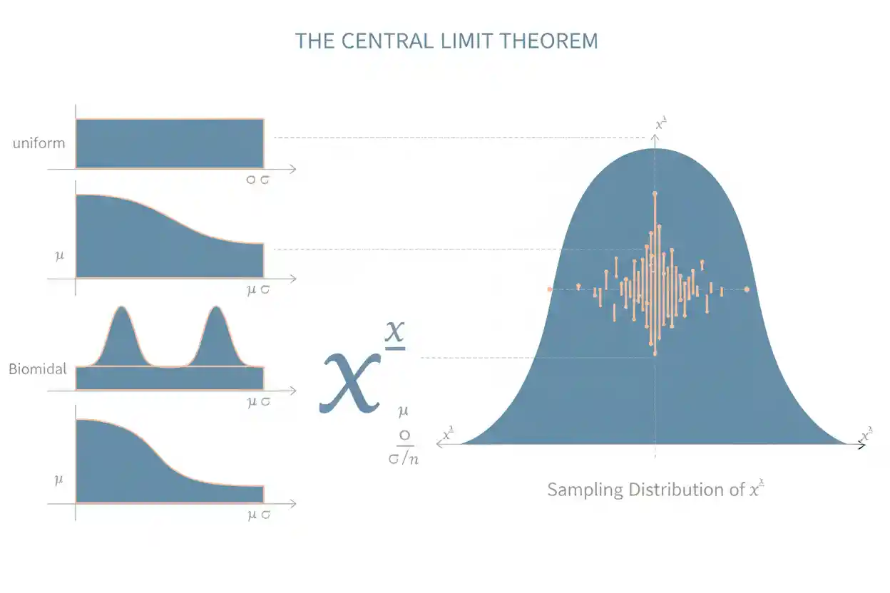
The central limit theorem is one of the most important results in probability and statistics because it explains why normal-distribution methods work in many situations even when the original population is not normally distributed. In its classical form, the theorem states that if independent and identically distributed random variables have a finite mean and finite variance, then the properly standardized sum—or equivalently the standardized sample mean—approaches a standard normal distribution as the sample size becomes large. The crucial point is that the theorem describes the distribution of a statistic across repeated samples, not the shape of the raw observations themselves. A strongly skewed population does not become normally distributed simply because more observations are collected; rather, the distribution of sample means often becomes increasingly normal in shape as each sample contains more observations.
This distinction is fundamental to understanding sampling distributions and the role of the theorem in statistical inference. The central limit theorem helps justify normal approximations, standard-error calculations, confidence intervals, and many hypothesis-testing procedures. Its usefulness, however, depends on its assumptions and on how quickly convergence occurs for the population being studied. There is therefore no universal sample-size threshold that guarantees a good normal approximation in every problem.
The theorem belongs to the broader study of Statistics & Probability and is especially important within Inference & Regression, where researchers use sample information to reason about unknown population quantities.
What Is the Central Limit Theorem?
Suppose X₁, X₂, …, Xₙ are independent observations from the same population distribution. Assume that this population has mean μ and finite variance σ². The sample mean x̄ is calculated by adding the observations and dividing by the sample size. If many independent samples of size n were repeatedly drawn from the same population and the mean were calculated for every sample, those means would form a sampling distribution. The central limit theorem says that, under the classical conditions, the standardized sampling distribution of x̄ approaches the standard normal distribution as n increases.
x̄ = Σxᵢ / n
For independent and identically distributed observations with population mean μ and population standard deviation σ:
E(x̄) = μ
and
SE(x̄) = σ / √n
The first equation says that the expected value of the sample mean equals the population mean. In other words, x̄ is an unbiased estimator of μ under ordinary random-sampling conditions. The second equation describes the spread of the sampling distribution of x̄. This spread is the standard error, and it decreases as the sample size increases because √n appears in the denominator.
The central limit theorem then concerns the standardized quantity:
Zₙ = (x̄ − μ) / (σ / √n)
As n becomes large, the distribution of Zₙ approaches the standard normal distribution, whose mean is 0 and whose standard deviation is 1. Symbolically, this is often described by saying that Zₙ converges in distribution to N(0, 1).
The Central Limit Theorem Is About Sampling Distributions
One of the most common misunderstandings is that the central limit theorem makes the original data normal. It does not. Consider a population of customer waiting times that is strongly right-skewed because most customers are served quickly while a small number wait much longer. Drawing a sample of 100 customers does not make those 100 individual waiting times normally distributed. Their distribution may remain noticeably skewed.
What changes is the distribution obtained by repeatedly taking samples of 100 customers and calculating a mean for each sample. Those sample means tend to cluster around the population mean, and their distribution generally becomes more symmetric and normal-looking as the sample size increases. The distinction between the distribution of observations and the distribution of a statistic is central to statistical reasoning. A broader treatment of how statistics behave across repeated samples appears in the discussion of sampling distributions.
For the sample mean, three quantities are especially important: the center of the sampling distribution, its spread, and its shape. The center is μ, the standard error is σ/√n, and the central limit theorem provides an increasingly useful normal approximation to the shape under appropriate conditions.
Why the Sample Mean Becomes More Stable
A sample mean combines information from many observations. Individual observations can vary substantially, but positive and negative deviations from the population mean partly offset one another when averaged. Consequently, the variability of x̄ is smaller than the variability of individual observations.
If the population standard deviation is σ, then:
SE(x̄) = σ / √n
Suppose σ = 20. For samples of size n = 25:
SE(x̄) = 20 / √25 = 4
For samples of size n = 100:
SE(x̄) = 20 / √100 = 2
Increasing the sample size from 25 to 100 reduces the standard error from 4 to 2. The sample size became four times as large, but the standard error became only half as large because precision improves according to √n rather than n itself. This square-root relationship has an important practical implication: obtaining twice the precision typically requires roughly four times the sample size, assuming the other conditions remain unchanged.
The Classical Independent, Identically Distributed Case
The simplest and most commonly taught version of the central limit theorem assumes that X₁, X₂, …, Xₙ are independent and identically distributed, usually abbreviated i.i.d. Each observation therefore comes from the same population distribution, and knowing one observation does not determine another. The variables are also assumed to have a finite population mean μ and finite variance σ².
Under these conditions, define:
Sₙ = ΣXᵢ
The expected value of the sum is:
E(Sₙ) = nμ
Its standard deviation is:
SD(Sₙ) = σ√n
The standardized sum can therefore be written as:
Zₙ = (Sₙ − nμ) / (σ√n)
As n increases, the distribution of this standardized sum approaches N(0, 1). Since x̄ = Sₙ/n, the sum form and sample-mean form describe the same underlying convergence from two different perspectives.
The theorem has broader versions that relax identical-distribution assumptions and allow certain forms of dependence, but those extensions require additional mathematical conditions. The classical i.i.d. finite-variance version is the appropriate foundation for most introductory applications and should not be generalized casually to situations where the assumptions are badly violated.
Worked Example: Sample Mean
Suppose the individual transaction values generated by a process have population mean μ = 80 and population standard deviation σ = 24. The individual transaction distribution is moderately right-skewed. A researcher takes random independent samples of n = 64 transactions and calculates the sample mean for each sample.
The expected value of the sample mean is:
E(x̄) = μ = 80
Its standard error is:
SE(x̄) = 24 / √64
SE(x̄) = 24 / 8 = 3
Therefore, the sampling distribution of x̄ is centered at 80 and has a standard deviation of 3. If n = 64 is sufficiently large for the amount of skewness present, the central limit theorem allows the sampling distribution of x̄ to be approximated by a normal distribution.
Suppose one particular sample produces x̄ = 86. Its standardized value is:
Z = (86 − 80) / 3
Z = 2
The observed sample mean lies two standard errors above the population mean. Interpreting a standardized value in detail belongs to the broader concept of the z-score; in the central limit theorem context, the important point is that the theorem explains why a normal reference distribution can often be used for this standardized sample mean.
Central Limit Theorem for Sums
The theorem applies just as naturally to sums as to averages. Suppose X represents the amount spent by one randomly selected customer, with mean μ = 50 and standard deviation σ = 12. If 100 independent customers are considered, their total spending is:
S₁₀₀ = X₁ + X₂ + … + X₁₀₀
Its expected value is:
E(S₁₀₀) = 100 × 50 = 5,000
Its standard deviation is:
SD(S₁₀₀) = 12√100 = 120
Even if individual spending is not normally distributed, the distribution of total spending across many independent groups of 100 customers may be well approximated by a normal distribution when the conditions are suitable.
This sum-based interpretation is useful whenever a problem involves aggregate demand, total claims, accumulated measurements, total production, or another quantity formed by adding many individual random contributions.
Effect of Increasing the Sample Size
Increasing n has two distinct effects on the sampling distribution of the sample mean. First, its standard error becomes smaller because σ/√n decreases. Sample means therefore become more tightly concentrated around μ. Second, under the central limit theorem, the standardized sampling distribution generally becomes closer to the standard normal distribution.
These two effects should not be confused. The narrowing of the sampling distribution follows directly from the variance of the mean under independence, while the improvement in normal approximation comes from the limiting behavior described by the theorem. A sample mean can become more precise as n grows even before its sampling distribution is particularly close to normal.
How quickly normality emerges depends strongly on the underlying population distribution. A population that is already normal requires no asymptotic approximation for the sample mean: if observations are independent and normally distributed, x̄ is exactly normal for every positive sample size. A reasonably symmetric, light-tailed non-normal population may produce a useful approximation at relatively modest n. A heavily skewed or heavy-tailed population may require substantially larger samples.
Why “n = 30” Is Not a Universal Rule
The claim that the central limit theorem automatically applies whenever n ≥ 30 is an oversimplification. Thirty observations can be adequate for some populations and inadequate for others. There is no universal value of n at which every possible finite-variance population suddenly produces an accurately normal sampling distribution.
For a nearly symmetric population without extreme tails, samples smaller than 30 may already yield a reasonable approximation for the mean. For a severely right-skewed distribution with rare extreme observations, even samples much larger than 30 can retain noticeable skewness in the sampling distribution. The approximation quality depends on features such as skewness, tail behavior, outliers, and the particular level of accuracy required by the analysis.
Sample size should therefore be evaluated together with the shape and behavior of the underlying data-generating process. Treating 30 as an automatic pass/fail threshold ignores the actual mathematics of convergence.
Skewed Populations and Convergence Speed
Skewness does not invalidate the central limit theorem merely because the population is non-normal. In fact, one of the theorem’s major advantages is that it can produce approximately normal sampling distributions from non-normal populations. However, strong skewness can slow convergence.
Imagine a population in which most observations are between 0 and 10 but occasional values exceed 1,000. Small samples may or may not contain one of these extreme observations. As a result, their sample means can vary substantially and the sampling distribution may remain asymmetric. Larger samples spread the effect of extreme observations across more data points, generally making the mean more stable, but convergence can still be slow.
The practical conclusion is not that skewed data prohibit the theorem. Rather, stronger skewness and more extreme tails usually require greater caution when deciding whether the normal approximation is accurate enough for the intended application.
Heavy Tails and the Finite-Variance Requirement
The classical theorem assumes finite variance. This requirement matters because the normalization σ/√n depends on σ being finite. Some theoretical probability distributions have such heavy tails that their variance is infinite or undefined. For those distributions, the ordinary classical central limit theorem does not apply in the usual form.
This is different from merely having a large population variance. A distribution can have high variability while still possessing a finite variance, in which case the classical theorem may remain applicable. The key mathematical issue is whether the required moments actually exist.
Heavy-tailed practical data can also create problems even when the true variance is technically finite. Rare extreme observations may cause slow convergence and unstable finite-sample behavior. Therefore, analysts should distinguish the asymptotic theorem—what happens as n approaches infinity—from the quality of an approximation at the sample size actually available.
Central Limit Theorem vs the Normal Distribution
The normal distribution is a probability distribution. The central limit theorem is a theorem about the limiting distribution of standardized sums or means under specified conditions. These concepts are closely connected but not interchangeable.
A population can itself be normal. In that special case, independent sample means are exactly normal regardless of sample size. Alternatively, a population can be uniform, skewed, discrete, or otherwise non-normal, yet the sampling distribution of its mean may become approximately normal as n increases. The theorem explains this second phenomenon.
It is therefore incorrect to say that the central limit theorem states that “large samples are normal.” A sample is simply a collection of observations. The theorem concerns a standardized statistic viewed across repeated hypothetical samples.
Central Limit Theorem vs Law of Large Numbers
The central limit theorem and the Law of Large Numbers both describe what happens as sample size increases, but they answer different questions. The Law of Large Numbers says, roughly, that the sample mean tends toward the population mean as more observations are collected. It therefore concerns convergence of the estimator toward the true value.
The central limit theorem goes further in a different direction: it describes the shape and scale of the random fluctuations around μ. Specifically, it explains why the appropriately standardized difference between x̄ and μ often approaches a normal distribution.
A useful distinction is:
Law of Large Numbers: x̄ tends toward μ.
Central Limit Theorem: the standardized fluctuations of x̄ around μ tend toward a normal distribution under suitable conditions.
The first statement explains consistency. The second provides a distributional approximation that can be used to quantify uncertainty.
Central Limit Theorem for Sample Proportions
A sample proportion can be viewed as a sample mean of Bernoulli random variables. Suppose Xᵢ = 1 when an observation has a particular characteristic and Xᵢ = 0 otherwise. If the population probability of the characteristic is p, then each Xᵢ has expected value p, and the sample proportion is:
p̂ = ΣXᵢ / n
Its expected value is:
E(p̂) = p
Its standard error is:
SE(p̂) = √[p(1 − p) / n]
Because p̂ is an average of Bernoulli variables, the central limit theorem provides the theoretical foundation for approximating its sampling distribution by a normal distribution when the sample is sufficiently informative and observations satisfy the relevant independence conditions.
For finite samples, however, the quality of the approximation depends strongly on p and n. When p is extremely close to 0 or 1, the distribution of the number of successes can remain strongly asymmetric unless n is large. The exact count of successes follows a binomial distribution when the standard Bernoulli-trial assumptions hold, so a normal approximation should not automatically replace the exact model in small or highly unbalanced cases.
Normal Approximation to a Probability
Consider a process in which individual observations have μ = 40 and σ = 10. Suppose independent samples of n = 100 are taken. We want to understand the approximate probability that a sample mean is greater than 42.
First calculate the standard error:
SE(x̄) = 10 / √100 = 1
Then standardize 42:
Z = (42 − 40) / 1 = 2
If the central limit theorem provides a sufficiently accurate approximation, the required probability can be approximated using the upper tail of the standard normal distribution beyond Z = 2. The theorem does not itself supply the numerical tail probability; it justifies using the normal reference distribution for the standardized mean under suitable conditions.
This distinction is useful. The central limit theorem establishes an approximation framework, while normal-distribution calculations determine the corresponding approximate probabilities.
Connection to Confidence Intervals
Many confidence intervals are built by combining a point estimate with a measure of its sampling variability. For a sample mean with known population standard deviation, the central limit theorem supports an approximate normal model for the standardized error when the sample size is sufficiently large and the assumptions are appropriate.
Conceptually, the construction follows the pattern:
estimate ± critical value × standard error
The central limit theorem explains why a normal critical value can often be meaningful for sample means even when the original population itself is not normal. The interval, however, should not be interpreted as assigning a frequentist probability to the fixed population parameter after the data have been observed. A 95% frequentist confidence procedure is designed so that, under repeated sampling and the model assumptions, 95% of intervals constructed by that procedure would contain the true parameter.
The quality of the approximation still depends on the sampling process, sample size, population behavior, and whether nuisance quantities such as σ must be estimated.
Connection to Hypothesis Testing
The theorem also underlies many large-sample testing procedures. Suppose a test compares an observed sample mean with a value specified under a null hypothesis. If the standardized sample statistic has an approximately normal sampling distribution under H₀, the observed statistic can be compared with that reference distribution.
The competing claim may be represented by an alternative hypothesis. A resulting p-value measures how extreme the observed result, or a more extreme result under the test definition, would be if the null model were true. It is not the probability that H₀ itself is true.
The central limit theorem therefore helps provide a distributional foundation for some large-sample tests, but it does not determine whether an observed effect is practically important. Statistical significance and practical importance remain separate questions.
Independence Matters
The classical central limit theorem assumes independence. If observations are strongly dependent, the usual standard-error formula may be wrong and the standard i.i.d. version of the theorem may not justify a normal approximation.
For example, daily measurements in a time series may be correlated with nearby days. Measurements from people in the same household, students in the same classroom, or patients treated at the same clinic may also be clustered. Treating such observations as independent can underestimate uncertainty because the sample may contain less independent information than its nominal size suggests.
There are central limit theorems for various dependent processes, but they require their own assumptions. The existence of those extensions does not justify applying the ordinary formula σ/√n blindly to correlated observations.
Identically Distributed Observations
The classical version also assumes observations come from the same distribution. In practice, this may be questionable when observations come from different subpopulations, different measurement regimes, or processes that change over time.
More general forms of the theorem can handle independent but non-identically distributed variables when suitable conditions limit the contribution of individual terms. Nevertheless, analysts should not treat every heterogeneous collection of observations as if it were automatically covered by the simplest i.i.d. statement.
The practical task is to understand how the data were generated. Mathematical approximation is strongest when the assumptions correspond reasonably well to that process.
When the Central Limit Approximation Can Be Poor
A large sample does not guarantee that every normal approximation is accurate. Approximation can be poor when the population is extremely skewed, observations have very heavy tails, individual observations can dominate the sum, the sample remains too small relative to the population’s irregularity, dependence is strong, or the variance required by the classical theorem does not exist.
Rare-event proportions are another common problem. If p is very small and n is not large enough to generate a reasonable number of expected successes, the distribution of p̂ can remain highly asymmetric. Likewise, a sample mean calculated from a population containing extremely rare but enormous values may converge slowly.
The central limit theorem is an asymptotic result. It describes limiting behavior as n grows, while real analyses are performed at finite sample sizes. Good statistical practice therefore asks not only whether the theorem applies in principle, but also whether its approximation is sufficiently accurate for the particular decision being made.
Worked Example With a Skewed Population
Suppose the population distribution of order values has mean μ = 120 and standard deviation σ = 90, but the distribution is strongly right-skewed because a small fraction of orders are exceptionally large. A business takes random independent samples of n = 225 orders.
The expected sample mean is:
E(x̄) = 120
The standard error is:
SE(x̄) = 90 / √225
SE(x̄) = 90 / 15 = 6
Thus the sample means are centered at 120 with standard deviation 6. The original order values may remain extremely skewed, but the distribution of means across repeated samples of 225 orders can be much more symmetric.
Suppose a sample produces x̄ = 132:
Z = (132 − 120) / 6
Z = 2
The observed mean is two standard errors above the population mean. Whether the normal approximation is sufficiently accurate still depends on the severity of the original skewness and tail behavior. The calculation demonstrates the mechanics of the theorem but does not prove that n = 225 is adequate for every possible skewed population.
A Second Worked Example: Sample Proportion
Suppose 40% of a very large population has a particular binary characteristic, so p = 0.40. A random independent sample of n = 400 is selected.
The expected sample proportion is:
E(p̂) = 0.40
The standard error is:
SE(p̂) = √[0.40(1 − 0.40) / 400]
SE(p̂) = √(0.24 / 400)
SE(p̂) = √0.0006
SE(p̂) ≈ 0.0245
The sampling distribution of p̂ is therefore centered at 0.40 with an approximate standard deviation of 0.0245. Because the sample contains substantial expected counts in both outcome categories, a normal approximation is generally much more plausible here than it would be for an extremely rare outcome.
If the observed sample proportion were 0.449:
Z ≈ (0.449 − 0.40) / 0.0245
Z ≈ 2.00
Again, the central limit theorem supplies the large-sample distributional reasoning. The exact interpretation of a particular test or interval depends on the statistical procedure being used.
Central Limit Theorem and Standard Error
The central limit theorem and standard error are closely connected but describe different things. The standard error measures the standard deviation of a statistic’s sampling distribution. For the sample mean in the classical independent case with known σ:
SE(x̄) = σ / √n
The central limit theorem concerns the shape of the standardized distribution as n grows. Consequently, knowing the standard error tells us how widely sample means vary, while the theorem tells us why their standardized distribution can often be approximated by a normal curve.
This distinction is useful because a standard error can exist even when the finite-sample distribution is not close to normal. Precision and approximate normality are related but separate properties.
Where the Central Limit Theorem Fits in Statistical Inference
Statistical inference includes many tools, and the central limit theorem provides foundational reasoning for some of them rather than replacing them. Procedures based on means and proportions often rely directly or indirectly on large-sample normal approximations. Other methods have different reference distributions and assumptions.
For example, a chi-square goodness of fit procedure evaluates whether observed categorical frequencies differ from specified expected frequencies, while a chi-square test of independence evaluates association between categorical variables in a contingency table. Those methods should be understood through their own test statistics and conditions rather than treated as applications of the sample-mean formula presented here.
Likewise, the coefficient of determination describes how much variation in an outcome is accounted for by a regression model, while Cohen’s d is an effect-size measure used to express a standardized difference. These quantities address different statistical questions. The central limit theorem’s role is narrower and more foundational: it explains an important limiting distribution for sums and averages.
Common Misconceptions
A frequent misconception is that any dataset with more than 30 observations is normally distributed. The central limit theorem says no such thing. Raw data can remain skewed, multimodal, discrete, or heavy-tailed regardless of sample size.
Another misconception is that n = 30 guarantees an accurate normal approximation. Approximation quality depends on the underlying population, and convergence can be fast or slow. Thirty is at most a rough teaching convention in some settings, not a theorem.
A third mistake is assuming that the theorem removes the need for independence. Large samples do not automatically repair strong dependence. If the observations are correlated, the usual standard-error formula can be substantially incorrect.
It is also incorrect to conclude that all statistics become normally distributed. The classical theorem applies directly to properly standardized sums and averages under its assumptions. Some other statistics have asymptotic normal distributions, but that requires separate results.
Finally, the theorem should not be interpreted as proof that an approximate method is sufficiently accurate for every practical purpose. An approximation that is adequate for a rough descriptive calculation may not be adequate for a highly sensitive tail-probability calculation.
Practical Checklist for Applying the Central Limit Theorem
Before relying on the theorem, identify exactly what quantity is being approximated. If the target is a mean or sum, determine whether the observations can reasonably be treated as independent, whether they arise from a sufficiently stable population, and whether the population has finite variance. Examine whether the data-generating process is highly skewed, heavy-tailed, dominated by rare extreme values, or clustered.
Next, consider the sample size in relation to those features rather than relying on a universal cutoff. Calculate the appropriate expected value and standard error, then standardize the statistic if a normal approximation is required. If the statistic is a proportion, remember that the behavior of the approximation depends on both n and p, not on n alone.
Finally, distinguish the mathematical approximation from the inference performed with it. A normal approximation may justify a reference distribution, but a confidence interval, hypothesis test, effect-size calculation, or regression result still has its own interpretation and assumptions.
Frequently Asked Questions
What does the central limit theorem say in simple terms?
It says that under appropriate conditions, the distribution of properly standardized sums or sample means becomes increasingly close to a normal distribution as sample size grows, even when the underlying population itself is not normal.
Does the central limit theorem mean the data become normally distributed?
No. The raw observations do not become normal merely because the sample is large. The theorem concerns the sampling distribution of a standardized sum or mean across repeated samples.
What is the formula for the sample mean?
For observations x₁, x₂, …, xₙ:
x̄ = Σxᵢ / n
The sample mean is the arithmetic average of the observations.
What is the expected value of the sample mean?
If each observation has population mean μ:
E(x̄) = μ
Thus, under the standard sampling assumptions, the sample mean is centered on the population mean.
What is the standard error of the sample mean?
For independent observations with population standard deviation σ:
SE(x̄) = σ / √n
The sampling variability decreases as sample size increases.
Is n = 30 always enough for the central limit theorem?
No. There is no universal n = 30 rule. Smaller samples can work well for symmetric, light-tailed populations, while substantially larger samples may be necessary for highly skewed or heavy-tailed populations.
Does the population have to be normally distributed?
No. That is one of the main reasons the theorem is useful. Under appropriate assumptions, the sampling distribution of the mean can approach normality even when the population is non-normal. If the population is normal, however, the sample mean is already normally distributed under independent sampling.
What happens as sample size increases?
The standard error of the sample mean decreases at the rate 1/√n, and the standardized sampling distribution generally moves closer to a standard normal distribution under the theorem’s conditions.
What is the difference between the central limit theorem and the Law of Large Numbers?
The Law of Large Numbers describes the sample mean approaching the population mean. The central limit theorem describes the distribution of the standardized random fluctuations around that population mean.
Does the central limit theorem apply to proportions?
Yes. A sample proportion is an average of Bernoulli variables, so the theorem can justify a normal approximation when the relevant assumptions hold and the sample provides enough information for the approximation to be accurate.
Does independence matter?
Yes. Independence is part of the classical i.i.d. theorem. Some extensions permit dependence under additional conditions, but the ordinary independent-sample formulas should not automatically be applied to correlated observations.
Why is finite variance important?
The classical theorem uses σ to scale the sum or mean. If the population variance is infinite or undefined, the ordinary finite-variance central limit theorem does not apply in its standard form.
Can the central limit theorem be used for confidence intervals?
Yes. It helps justify normal approximations used in many large-sample confidence interval procedures. The exact interval still depends on the parameter, estimator, standard-error calculation, and assumptions involved.
Does a normal approximation guarantee an accurate p-value?
No. The approximation must be sufficiently accurate in the region of the distribution relevant to the test. Tail probabilities can be sensitive to approximation error, especially with skewed, heavy-tailed, dependent, or small-sample data.
Key Takeaway
The central limit theorem explains why sums and averages occupy such a central position in statistical inference. For independent, identically distributed random variables with finite mean μ and finite variance σ², the standardized sample mean approaches a standard normal distribution as sample size increases:
Zₙ = (x̄ − μ) / (σ / √n)
The theorem does not say that raw data become normal, that every statistic becomes normally distributed, or that 30 observations are always sufficient. It provides an asymptotic description of a sampling distribution, and the speed of convergence depends on the underlying population. Used with appropriate attention to independence, finite variance, skewness, tail behavior, and sample size, it gives a powerful mathematical basis for normal approximations and many procedures used throughout statistical inference.



