


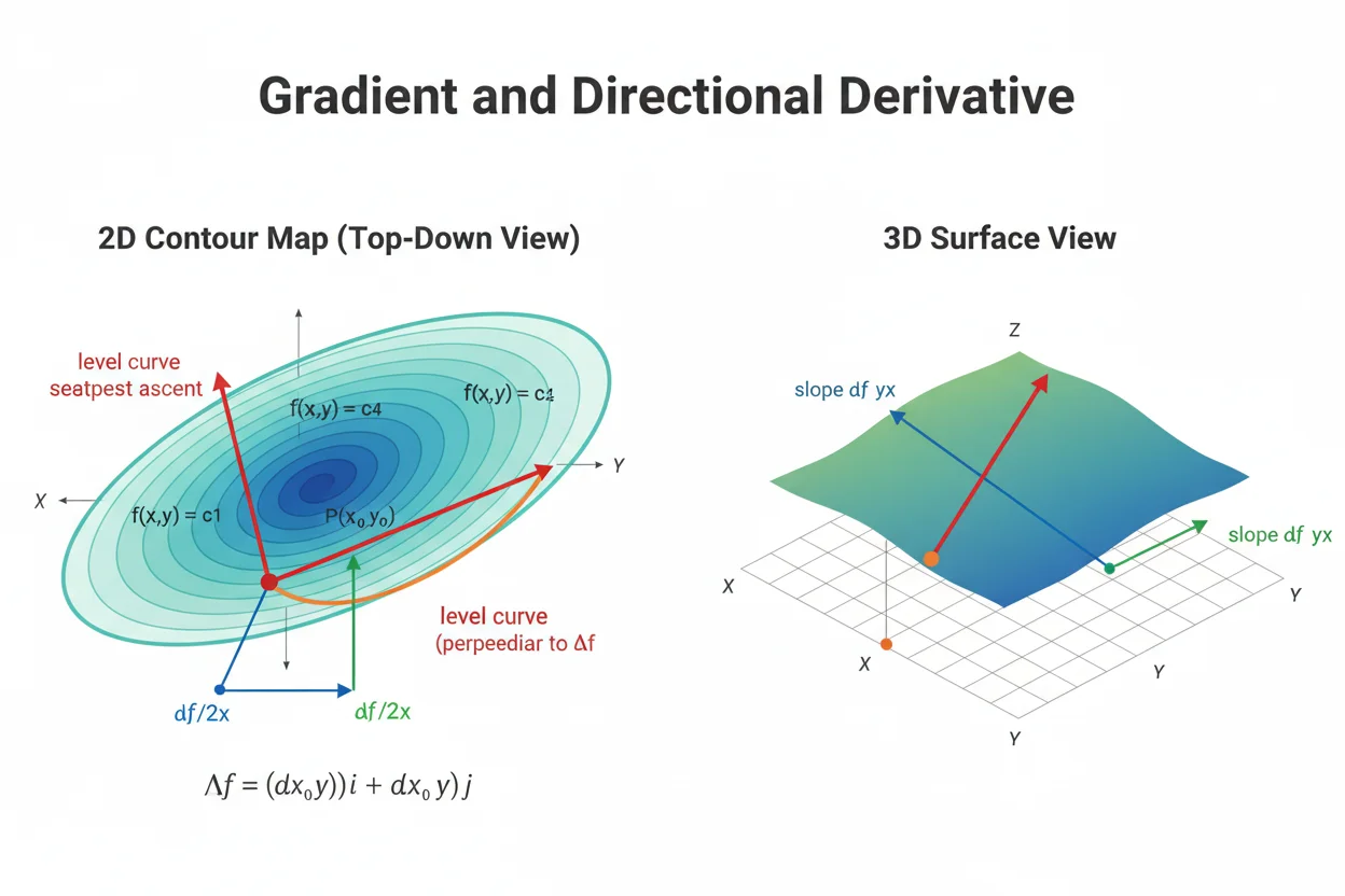
The gradient is a vector containing the first partial derivatives of a scalar-valued function. For a function f(x, y), the gradient is ∇f = (∂f/∂x, ∂f/∂y), while for f(x, y, z) it has three components. Geometrically, the gradient points in the direction of the greatest local increase of the function, and its magnitude gives the maximum rate of increase per unit distance. At a regular point, the gradient is perpendicular to a level curve or level surface. The gradient also determines every directional derivative through Dᵤf = ∇f · u, where u is a unit direction vector. If the gradient is zero, the point is stationary to first order, although that alone does not prove a maximum or minimum. Calculating a gradient therefore requires finding the relevant partial derivatives and evaluating them at the point of interest. The concept is central to multivariable calculus, optimization, geometry, physical fields, and mathematical models involving change across several directions.
What Is a Gradient?
Suppose:
f(x, y)
is a scalar-valued function of two variables.
Its gradient is:
∇f = (fₓ, fᵧ)
where:
fₓ = ∂f/∂x
and:
fᵧ = ∂f/∂y
In three variables:
f(x, y, z)
the gradient is:
∇f = (fₓ, fᵧ, f_z)
The result is a vector, even though f itself produces scalar values.
This vector summarizes the function’s first-order local change in all coordinate directions.
Gradient Formula
For two variables:
∇f(x, y) = (∂f/∂x, ∂f/∂y)
For three variables:
∇f(x, y, z) = (∂f/∂x, ∂f/∂y, ∂f/∂z)
More generally, for:
f(x₁, x₂, …, xₙ)
the gradient is:
∇f = (∂f/∂x₁, ∂f/∂x₂, …, ∂f/∂xₙ)
Every component is an ordinary partial derivative with respect to one independent variable.
How to Find a Gradient
Consider:
f(x, y) = x² + 3xy + 2y²
Differentiate with respect to x while treating y as constant:
fₓ = 2x + 3y
Differentiate with respect to y while treating x as constant:
fᵧ = 3x + 4y
Therefore:
∇f(x, y) = (2x + 3y, 3x + 4y)
At:
(1, 2)
we obtain:
∇f(1, 2) = (2 + 6, 3 + 8)
= (8, 11)
So the gradient at (1, 2) is:
(8, 11)
What Does the Gradient Mean?
The gradient has both direction and magnitude.
Its direction gives the direction in the input space in which the function increases most rapidly.
Its magnitude:
|∇f|
gives the maximum local rate of increase per unit distance.
For:
∇f(1, 2) = (8, 11)
the magnitude is:
|∇f| = √(8² + 11²)
= √185
≈ 13.60
Therefore the maximum local rate of increase at that point is approximately:
13.60
Direction of Steepest Increase
If:
∇f ≠ 0
then the unit direction of steepest increase is:
u_max = ∇f/|∇f|
For:
∇f = (8, 11)
we get:
u_max = (8/√185, 11/√185)
Moving initially in this direction increases f more rapidly than moving in any other unit direction.
The maximum rate is:
D_max f = |∇f|
Direction of Steepest Decrease
The direction of steepest decrease is opposite the gradient:
u_min = −∇f/|∇f|
The minimum directional derivative is:
D_min f = −|∇f|
For:
∇f = (8, 11)
the steepest-descent direction is:
(−8/√185, −11/√185)
and the corresponding rate is:
−√185
Gradient and Directional Derivative
The directional derivative of f in a unit direction u is:
Dᵤf = ∇f · u
where · is the dot product.
If θ is the angle between the gradient and u:
Dᵤf = |∇f| cos θ
This formula explains the geometric role of the gradient.
When:
θ = 0°
the direction agrees with the gradient and the rate is maximal.
When:
θ = 180°
the direction is opposite the gradient and the rate is most negative.
When:
θ = 90°
the directional derivative is zero.
Directional Derivative Example
Suppose:
∇f(1, 2) = (8, 11)
and the unit direction is:
u = (3/5, 4/5)
Then:
Dᵤf = (8, 11) · (3/5, 4/5)
= 24/5 + 44/5
= 68/5
= 13.6
In this case, the chosen direction is very close to the gradient direction, so the directional rate is close to the maximum possible value.
Gradient and Level Curves
A level curve of f(x, y) is defined by:
f(x, y) = c
where c is constant.
At a regular point where:
∇f ≠ 0
the gradient is perpendicular to the level curve.
Why? Moving tangentially along a level curve does not change f to first order.
If t is a tangent unit vector, then:
Dₜf = 0
But:
Dₜf = ∇f · t
Therefore:
∇f · t = 0
so the gradient and tangent direction are perpendicular.
Example With a Circle
Consider:
f(x, y) = x² + y²
The level curves are:
x² + y² = c
which are circles centered at the origin.
The gradient is:
∇f = (2x, 2y)
At:
(3, 4)
we have:
∇f = (6, 8)
This vector points radially outward from the origin.
That makes geometric sense because the radial direction is perpendicular to the circle passing through (3, 4).
Gradient and Level Surfaces
For a function of three variables:
f(x, y, z)
a level surface is:
f(x, y, z) = c
At a regular point, the gradient:
∇f = (fₓ, fᵧ, f_z)
is normal to that surface.
Therefore a normal vector to a level surface can often be found immediately by evaluating the gradient.
This is one of the most important geometric applications of the gradient.
Example: Normal Vector to a Surface
Consider the surface:
x² + y² + z² = 25
Define:
f(x, y, z) = x² + y² + z²
Then:
∇f = (2x, 2y, 2z)
At:
(3, 4, 0)
the gradient is:
∇f(3, 4, 0) = (6, 8, 0)
Therefore:
(6, 8, 0)
is a normal vector to the sphere at that point.
Any nonzero scalar multiple, such as:
(3, 4, 0)
is also a valid normal direction.
Gradient in Three Variables
Let:
f(x, y, z) = x²y + yz³ + 4x
Find the gradient.
Differentiate with respect to x:
fₓ = 2xy + 4
Differentiate with respect to y:
fᵧ = x² + z³
Differentiate with respect to z:
f_z = 3yz²
Therefore:
∇f = (2xy + 4, x² + z³, 3yz²)
At:
(1, 2, 1)
we get:
∇f = (2·1·2 + 4, 1² + 1³, 3·2·1²)
= (8, 2, 6)
Gradient Magnitude
For:
∇f = (a, b)
the magnitude is:
|∇f| = √(a² + b²)
In three dimensions:
|∇f| = √(a² + b² + c²)
This magnitude is the maximum directional derivative at the point.
If:
∇f = 0
then:
|∇f| = 0
and every directional derivative predicted by the gradient formula is zero.
What Does a Zero Gradient Mean?
If:
∇f(a, b) = (0, 0)
then all first partial derivatives vanish at the point.
This makes:
(a, b)
a stationary or critical point when it lies in the interior of the domain and the necessary differentiability conditions hold.
However, a zero gradient does not by itself identify the point as a maximum or minimum.
The point could be:
- a local maximum,
- a local minimum,
- a saddle point,
- or another degenerate stationary point.
Further analysis is needed.
Example of a Minimum
Consider:
f(x, y) = x² + y²
Its gradient is:
∇f = (2x, 2y)
Set the gradient equal to zero:
2x = 0
2y = 0
So:
(x, y) = (0, 0)
At this point:
f(0, 0) = 0
and since:
x² + y² ≥ 0
for all real x and y, the point is a global minimum.
Example of a Saddle Point
Consider:
f(x, y) = x² − y²
Its gradient is:
∇f = (2x, −2y)
Set:
∇f = 0
Then:
x = 0
y = 0
So (0, 0) is a critical point.
But along the x-axis:
f(x, 0) = x² ≥ 0
while along the y-axis:
f(0, y) = −y² ≤ 0
The function increases in one direction and decreases in another.
Therefore the zero-gradient point is a saddle point, not a maximum or minimum.
Gradient and Optimization
Finding points where:
∇f = 0
is a central first step in multivariable optimization.
For an unconstrained differentiable function, an interior local extremum usually satisfies this condition.
The gradient identifies where the first-order change disappears, but classifying the point requires additional information.
Therefore:
∇f = 0
is generally a necessary condition for an interior differentiable extremum, not a sufficient condition.
Gradient and Differentials
For a differentiable function:
z = f(x, y)
the total differential is:
dz = fₓ dx + fᵧ dy
Using the gradient:
∇f = (fₓ, fᵧ)
and displacement:
dr = (dx, dy)
the differentials relation can be written:
dz = ∇f · dr
This expresses the local output change as the dot product of the gradient with a small input displacement.
Gradient and Linear Approximation
Near:
(a, b)
a differentiable function satisfies approximately:
f(a + Δx, b + Δy)
≈ f(a, b) + fₓ(a, b)Δx + fᵧ(a, b)Δy
Using the gradient:
f(a + Δx, b + Δy)
≈ f(a, b) + ∇f(a, b) · (Δx, Δy)
This is the multivariable version of linear approximation.
The gradient supplies all first-order coefficients in the local tangent-plane model.
Example of Local Change
Let:
f(x, y) = x² + xy + y²
At:
(2, 1)
the gradient is:
∇f = (2x + y, x + 2y)
Therefore:
∇f(2, 1) = (5, 4)
Suppose:
Δx = 0.01
Δy = −0.02
Then the approximate change is:
Δf ≈ (5, 4) · (0.01, −0.02)
= 0.05 − 0.08
= −0.03
The function is predicted to decrease by approximately 0.03.
Gradient Versus Ordinary Derivative
For a one-variable function:
f(x)
there is only one independent input direction, so the local rate is described by:
f′(x)
For:
f(x, y)
there are infinitely many directions in which one can move from a point.
The gradient packages the coordinate-direction rates into one vector from which rates in arbitrary directions can be obtained.
Thus the gradient is a multivariable extension of derivative information, not simply another notation for f′(x).
Gradient Versus Partial Derivative
A partial derivative is one component of the gradient.
For:
f(x, y)
we have:
fₓ
and:
fᵧ
Separately, each measures change along one coordinate axis.
Together:
∇f = (fₓ, fᵧ)
The gradient therefore combines coordinate-wise rates into a geometric vector.
Gradient Versus Directional Derivative
The gradient is a vector.
The directional derivative is a scalar.
They are connected by:
Dᵤf = ∇f · u
The gradient contains enough first-order information to calculate the directional derivative for every unit vector u, provided the function is differentiable at the point.
This distinction prevents a common error of calling |∇f| the directional derivative in every direction. It is the directional derivative only in the steepest-ascent direction.
Gradient and the Fundamental Theorem of Calculus
The Fundamental Theorem Of Calculus describes the inverse relationship between one-variable differentiation and integration.
The gradient instead collects first derivatives of a multivariable scalar function.
The concepts share the broader theme of local change, but their formulas serve different purposes.
In advanced vector calculus, gradient fields and integrals can be connected through path-independence results and higher-dimensional analogues of the fundamental theorem.
Gradient and Implicit Differentiation
A level curve can be defined implicitly:
F(x, y) = c
If y is locally a function of x, implicit differentiation gives:
Fₓ + Fᵧ(dy/dx) = 0
So, when Fᵧ ≠ 0:
dy/dx = −Fₓ/Fᵧ
The gradient:
∇F = (Fₓ, Fᵧ)
is perpendicular to the same level curve.
Thus implicit slope and gradient geometry describe the same local curve from complementary perspectives.
Example: Gradient and Implicit Slope
Consider:
x² + y² = 25
Define:
F(x, y) = x² + y²
Then:
∇F = (2x, 2y)
At:
(3, 4)
the gradient is:
(6, 8)
This is normal to the circle.
Implicit differentiation gives:
2x + 2y(dy/dx) = 0
Therefore:
dy/dx = −x/y
At (3, 4):
dy/dx = −3/4
A tangent vector can be represented by:
(4, −3)
Check the dot product:
(6, 8) · (4, −3)
= 24 − 24
= 0
So the tangent vector is perpendicular to the gradient, exactly as expected.
Gradient and Double Integrals
A double integral accumulates a scalar function across a two-dimensional region:
∬ᴿ f(x, y) dA
The gradient instead describes how the scalar function changes locally from point to point.
For example, if T(x, y) represents temperature, then:
∇T
shows the direction of fastest temperature increase, while:
∬ᴿ T(x, y) dA
can contribute to an average-temperature calculation over a region.
One operation is local and differential; the other is accumulative.
Gradient and Line Integrals
A line integral accumulates along a path.
When a vector field is itself the gradient of a scalar function:
F = ∇φ
the field has special properties on suitable domains.
Integrating such a gradient field along a curve can often be reduced to endpoint values of the scalar potential φ.
This is a higher-dimensional echo of the connection between derivatives and integrals, but the specialist line-integral treatment owns the detailed calculation procedure.
Gradient and Improper Integrals
An improper integral concerns integration across infinite intervals or near singularities.
A gradient concerns multivariable differentiation.
They are distinct operations, although both may appear in the same advanced model.
For example, a scalar potential might have a gradient describing a force field while an integral involving that field requires convergence analysis near a singular point.
The presence of a gradient does not remove the need to check whether an improper integral converges.
Gradient in a First-Order Differential Equation
A scalar first-order linear differential equation has form:
y′ + P(x)y = Q(x)
and normally uses an integrating factor rather than a gradient.
Gradients become relevant when the state depends on several independent variables or when a multivariable scalar field is involved.
The two concepts can appear together in more advanced differential systems, but the ordinary integrating-factor method does not require computing ∇f.
Gradient and Euler’s Method
The Euler method approximates the evolution of a differential equation using local derivative information.
For a scalar ODE:
y′ = f(x, y)
the method uses:
yₙ₊₁ = yₙ + h f(xₙ, yₙ)
A gradient, by contrast, collects partial derivatives of a scalar field.
In multivariable numerical methods, gradients may supply the direction used in an iterative algorithm, while Euler’s method supplies time- or input-stepping for a differential equation.
They both use local derivative information but for different purposes.
Gradient Descent Interpretation
If the goal is to decrease a differentiable function locally, the direction:
−∇f
provides steepest first-order decrease.
A small update can therefore take the form:
xnew = xold − α∇f
where α > 0 controls the step length.
This follows directly from the fact that:
−∇f/|∇f|
is the unit direction with the most negative directional derivative.
Choosing an appropriate step length is a separate issue from calculating the gradient itself.
Units of a Gradient
Gradient components have units of:
output units / corresponding input units
If:
T(x, y)
measures temperature in °C and x and y are measured in meters, then:
∂T/∂x
and:
∂T/∂y
have units:
°C/m
The gradient magnitude also has units of temperature change per unit distance when the spatial coordinates share the same units.
This helps give physical meaning to gradient calculations.
Gradient of a Constant
If:
f(x, y) = c
then:
fₓ = 0
and:
fᵧ = 0
Therefore:
∇f = (0, 0)
A constant scalar field has no preferred direction of increase because its value is the same everywhere.
Gradient of a Linear Function
Let:
f(x, y) = ax + by + c
Then:
fₓ = a
fᵧ = b
Therefore:
∇f = (a, b)
The gradient is constant everywhere.
This matches the geometry of a plane: its steepness and steepest-ascent direction do not change from point to point.
Gradient of a Quadratic Function
Let:
f(x, y) = x² + 4xy + 3y²
Then:
fₓ = 2x + 4y
fᵧ = 4x + 6y
So:
∇f = (2x + 4y, 4x + 6y)
Unlike a linear function, the gradient changes with position.
This means both the steepest direction and maximum rate of increase vary across the surface.
Gradient and Continuity
A function can have partial derivatives at a point without necessarily being fully differentiable there.
When f is differentiable, the gradient provides the coefficients of its local linear approximation.
Differentiability also implies continuity at the point.
Therefore the standard geometric interpretations of the gradient are strongest when full differentiability has been established rather than when isolated partial derivatives merely happen to exist.
Gradient Within Multivariable Calculus
The gradient is one of the foundational tools of multivariable calculus.
It links partial derivatives, directional derivatives, level sets, tangent geometry, local approximation, and optimization.
It also interacts naturally with vector operations while remaining a derivative of a scalar field rather than an arbitrary vector calculation.
The broader Calculus & Linear Algebra framework provides the surrounding concepts without changing the gradient’s core role: summarizing first-order multivariable change.
Common Gradient Mistakes
One common error is returning a scalar instead of a vector. The gradient of a scalar function of several variables is a vector of partial derivatives.
Another mistake is differentiating all variables at once. For fₓ, other independent variables are treated as constants; for fᵧ, x is treated as constant.
Students also sometimes forget to evaluate every component at the requested point.
A frequent geometric mistake is saying that the gradient is tangent to a level curve. At regular points, the gradient is normal to the level curve or level surface.
A zero gradient should not automatically be labeled a minimum. Saddle points and maxima can also have zero gradients.
Finally, when finding a directional derivative from a gradient, the direction vector should normally be normalized first if the result is intended to measure change per unit distance.
Frequently Asked Questions
What is a gradient?
The gradient is the vector of first partial derivatives of a scalar-valued multivariable function.
For f(x, y):
∇f = (fₓ, fᵧ)
What is the gradient formula in three dimensions?
For f(x, y, z):
∇f = (fₓ, fᵧ, f_z)
Is a gradient a scalar or a vector?
It is a vector.
What direction does the gradient point?
When the gradient is nonzero, it points in the direction of greatest local increase of the function.
What does the magnitude of the gradient mean?
|∇f|
is the maximum directional derivative, or the greatest local rate of increase per unit distance.
What is the direction of steepest decrease?
It is opposite the gradient:
−∇f/|∇f|
when ∇f ≠ 0.
Why is the gradient perpendicular to level curves?
Moving tangent to a level curve produces zero first-order change in the function. Therefore the tangent direction has zero dot product with the gradient.
What does a zero gradient mean?
It means all first partial derivatives are zero. The point is stationary to first order, but additional analysis is needed to determine whether it is a maximum, minimum, saddle point, or another type of critical point.
How is the gradient related to a directional derivative?
For unit vector u:
Dᵤf = ∇f · u
How is a partial derivative different from a gradient?
A partial derivative is one component measuring change along a coordinate direction. The gradient combines all first partial derivatives into one vector.
Can a function have partial derivatives but no usable gradient interpretation?
The partial derivatives may exist even when the function is not fully differentiable. The strongest geometric gradient interpretation relies on differentiability.
How do you check a gradient calculation?
Differentiate the original function separately with respect to each independent variable, verify that other variables were held constant in each step, and then substitute the requested point into every component.




