


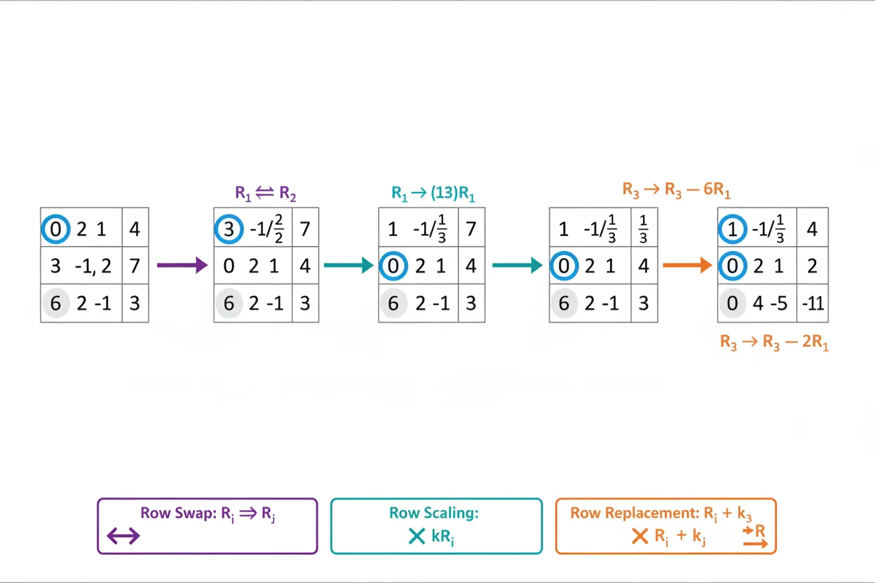
Row reduction is a systematic method for simplifying matrices through elementary row operations while preserving the solution set of the corresponding linear system. The three permitted operations are swapping two rows, multiplying a row by a nonzero scalar, and adding a multiple of one row to another. These operations can transform a complicated matrix into row echelon form or continue further to reduced row echelon form. Row reduction is used to solve systems of linear equations, identify pivot and free variables, calculate matrix rank, find inverses, determine consistency, and describe row and null spaces. The method is commonly associated with Gaussian elimination when elimination stops at echelon form and Gauss–Jordan elimination when reduction continues until every pivot column is cleared above and below its pivot. Although many valid sequences of row operations can be used, each individual operation must be applied to the entire row. Careful pivot selection and organized arithmetic are therefore more important than following one rigid sequence.
What Is Row Reduction?
Suppose a matrix is:
A = [ 1 2 ]
[ 3 4 ]
Row reduction changes A through valid elementary operations.
For example:
R₂ → R₂ − 3R₁
produces:
[ 1 2 ]
[ 0 −2 ]
The second matrix is row-equivalent to the first.
If the matrix represents a system of equations, both forms encode the same solution set.
This ability to simplify without changing the solutions is the central purpose of row reduction.
The Three Row Reduction Rules
Only three types of elementary row operation are needed.
Row Swap
Exchange two rows:
Rᵢ ↔ Rⱼ
For example:
[ 0 2 ]
[ 1 3 ]
can become:
[ 1 3 ]
[ 0 2 ]
by using:
R₁ ↔ R₂
Row swapping is useful when a better pivot is available in a lower row.
Row Scaling
Multiply an entire row by a nonzero scalar:
Rᵢ → cRᵢ
where:
c ≠ 0
For example:
[ 2 4 ]
can be scaled by 1/2:
R₁ → (1/2)R₁
to give:
[ 1 2 ]
Multiplication by zero is not allowed because it destroys information.
Row Replacement
Add a multiple of one row to another:
Rᵢ → Rᵢ + cRⱼ
For example:
R₂ → R₂ − 2R₁
can eliminate an entry below a pivot.
This is the operation used most frequently during elimination.
Why Elementary Row Operations Preserve Solutions
Consider the equations:
x + y = 5
2x − y = 1
The corresponding augmented matrix is:
[ 1 1 | 5 ]
[ 2 −1 | 1 ]
Replace the second equation by:
equation 2 − 2(equation 1)
This produces:
−3y = −9
or:
y = 3
No valid solution has been lost or introduced.
The matrix operation:
R₂ → R₂ − 2R₁
performs exactly the same algebra.
That is why row reduction can simplify a system of linear equations without changing its solution set.
Row Echelon Form
One common goal of row reduction is row echelon form.
A matrix is in row echelon form when:
- all zero rows are below nonzero rows,
- each pivot lies to the right of the pivot above it,
- all entries below each pivot are zero.
For example:
[ 1 2 3 ]
[ 0 1 4 ]
[ 0 0 5 ]
is in row echelon form.
The pivots are positioned like a staircase.
Back-substitution can then solve the corresponding system.
Reduced Row Echelon Form
Row reduction can continue until the matrix reaches Reduced Row Echelon Form.
In that form:
every pivot equals 1
and:
every pivot is the only nonzero entry in its column
For example:
[ 1 0 3 ]
[ 0 1 −2 ]
[ 0 0 0 ]
is reduced.
The dedicated RREF: Gauss–Jordan Elimination process focuses on carrying elimination all the way to this fully reduced form.
Gaussian Elimination Versus Gauss–Jordan Elimination
Gaussian elimination typically reduces a matrix to row echelon form.
The next step is usually back-substitution.
Gauss–Jordan elimination continues the row operations until reduced row echelon form is reached.
So the broad sequence is:
original matrix → echelon form → reduced echelon form
Gaussian elimination may stop after the first arrow.
Gauss–Jordan elimination continues through the second.
Both are row reduction methods.
Basic Row Reduction Example
Solve:
x + y = 5
2x − y = 1
Write the augmented matrix:
[ 1 1 | 5 ]
[ 2 −1 | 1 ]
Use:
R₂ → R₂ − 2R₁
Then:
[ 1 1 | 5 ]
[ 0 −3 | −9 ]
Scale the second row:
R₂ → −(1/3)R₂
giving:
[ 1 1 | 5 ]
[ 0 1 | 3 ]
At this point, back-substitution gives:
y = 3
and:
x + 3 = 5
so:
x = 2
Therefore:
(x, y) = (2, 3)
Continue to Reduced Form
Starting from:
[ 1 1 | 5 ]
[ 0 1 | 3 ]
use:
R₁ → R₁ − R₂
Then:
[ 1 0 | 2 ]
[ 0 1 | 3 ]
This is reduced row echelon form.
The solution is now visible directly:
x = 2
y = 3
No back-substitution is required.
Three-Variable Row Reduction Example
Solve:
x + y + z = 6
2x − y + z = 3
x + 2y − z = 2
Begin:
[ 1 1 1 | 6 ]
[ 2 −1 1 | 3 ]
[ 1 2 −1 | 2 ]
Use:
R₂ → R₂ − 2R₁
and:
R₃ → R₃ − R₁
giving:
[ 1 1 1 | 6 ]
[ 0 −3 −1 | −9 ]
[ 0 1 −2 | −4 ]
Swap rows 2 and 3:
R₂ ↔ R₃
Then:
[ 1 1 1 | 6 ]
[ 0 1 −2 | −4 ]
[ 0 −3 −1 | −9 ]
Now eliminate the entry beneath the second pivot:
R₃ → R₃ + 3R₂
giving:
[ 1 1 1 | 6 ]
[ 0 1 −2 | −4 ]
[ 0 0 −7 | −21 ]
Finish the Three-Variable Example
Scale row 3:
R₃ → −(1/7)R₃
Then:
[ 1 1 1 | 6 ]
[ 0 1 −2 | −4 ]
[ 0 0 1 | 3 ]
Back-substitution gives:
z = 3
From row 2:
y − 2(3) = −4
so:
y = 2
From row 1:
x + 2 + 3 = 6
so:
x = 1
Therefore:
(x, y, z) = (1, 2, 3)
Continuing elimination above the pivots would produce the identity matrix on the coefficient side.
Choosing a Pivot
A pivot is the entry used to eliminate other entries in its column.
Suppose the first column is:
[0]
[1]
[4]
Choosing the zero entry is impossible.
Swap the first row with the second row so that:
1
becomes the first pivot.
Even when the top entry is nonzero, another row may offer a simpler pivot and reduce arithmetic complexity.
Strategic row swaps can often avoid unnecessary fractions.
Pivot Positions
After elimination, pivots reveal the independent structure of the matrix.
For example:
[ 1 2 0 4 ]
[ 0 1 3 5 ]
[ 0 0 1 −2 ]
[ 0 0 0 0 ]
has three pivot positions.
Therefore the corresponding matrix rank is:
rank(A) = 3
Row reduction is one of the standard ways to calculate rank.
Free Variables
Consider:
[ 1 0 2 | 5 ]
[ 0 1 −3 | 1 ]
The first two columns contain pivots.
The third variable does not.
If the variables are:
x, y, z
then z is free.
The equations are:
x + 2z = 5
y − 3z = 1
Let:
z = t
Then:
x = 5 − 2t
y = 1 + 3t
The system has infinitely many solutions.
Row Reduction and Rank
The number of nonzero rows in echelon form equals the rank.
More precisely:
rank(A) = number of pivots
because row operations preserve linear dependence relationships.
For example:
A = [ 1 2 3 ]
[ 2 4 6 ]
[ 3 6 9 ]
reduces to:
[ 1 2 3 ]
[ 0 0 0 ]
[ 0 0 0 ]
Therefore:
rank(A) = 1
All three original rows were multiples of the same row direction.
Row Reduction and Matrix Inverses
Row reduction can calculate a matrix inverse.
For a square matrix A, construct:
[A | I]
and row-reduce the left side.
If the process reaches:
[I | B]
then:
B = A⁻¹
If the coefficient side cannot become I, the matrix is singular.
This method is particularly useful beyond the simplest 2×2 inverse formula.
Inverse Example
Let:
A = [ 2 1 ]
[ 1 1 ]
Start:
[ 2 1 | 1 0 ]
[ 1 1 | 0 1 ]
Swap:
R₁ ↔ R₂
giving:
[ 1 1 | 0 1 ]
[ 2 1 | 1 0 ]
Use:
R₂ → R₂ − 2R₁
Then:
[ 1 1 | 0 1 ]
[ 0 −1 | 1 −2 ]
Scale row 2 by −1:
[ 1 1 | 0 1 ]
[ 0 1 | −1 2 ]
Now:
R₁ → R₁ − R₂
giving:
[ 1 0 | 1 −1 ]
[ 0 1 | −1 2 ]
Therefore:
A⁻¹ = [ 1 −1 ]
[−1 2 ]
You can verify the result using matrix multiplication.
Row Reduction and the Determinant
The matrix determinant changes predictably under elementary row operations.
Swapping two rows multiplies the determinant by:
−1
Multiplying one row by c multiplies the determinant by:
c
Adding a multiple of one row to another leaves the determinant unchanged.
These rules allow a square matrix to be reduced to triangular form and its determinant obtained from the diagonal entries after accounting for swaps and row scalings.
Determinant Example by Reduction
Consider:
A = [ 1 2 3 ]
[ 2 5 7 ]
[ 1 0 4 ]
Use:
R₂ → R₂ − 2R₁
and:
R₃ → R₃ − R₁
giving:
[ 1 2 3 ]
[ 0 1 1 ]
[ 0 −2 1 ]
Then:
R₃ → R₃ + 2R₂
so:
[ 1 2 3 ]
[ 0 1 1 ]
[ 0 0 3 ]
Only row-replacement operations were used, so the determinant is unchanged.
Thus:
det(A) = 1·1·3
= 3
Row Reduction and Matrix Operations
Row reduction belongs to the broader family of matrix operations, but it differs from ordinary entrywise operations.
You do not simply change one matrix entry arbitrarily.
Every modification must act on a complete row according to one of the three elementary rules.
This is what preserves row equivalence and the solution structure of a linear system.
Elementary Matrices
Each elementary row operation can be represented by multiplication with an elementary matrix.
If E performs one row operation on A, then:
EA
is the transformed matrix.
A sequence of operations can therefore be written:
Eₖ…E₂E₁A
This creates a direct link between row reduction and matrix multiplication.
If the sequence reduces an invertible square matrix to I:
Eₖ…E₂E₁A = I
then:
Eₖ…E₂E₁ = A⁻¹
Row Reduction and Linear Transformations
A matrix can represent a linear transformation.
Row reduction preserves important structural information such as rank and null-space solutions, but the reduced matrix does not generally represent the identical geometric transformation.
Elementary row operations effectively modify the coordinate equations describing the output.
Therefore row-equivalent matrices should not automatically be interpreted as the same geometric mapping, even though they share important algebraic properties.
Row Reduction and Basis
Pivot columns identified during row reduction help construct bases.
If pivots occur in columns:
1, 3, and 4
then columns 1, 3, and 4 of the original matrix form a basis for its column space.
The ideas of basis and dimension explain why the number of pivot columns equals the dimension of that space.
For the row space, the nonzero rows of an echelon form can be used as a basis.
Homogeneous Systems
A homogeneous system has form:
Ax = 0
It is always consistent because:
x = 0
is a solution.
Row reduction determines whether nonzero solutions also exist.
If every variable column contains a pivot, only the trivial solution exists.
If there is at least one free variable, infinitely many solutions exist.
For an n×n matrix, a nontrivial homogeneous solution implies the matrix is singular.
Example of a Homogeneous System
Consider:
[ 1 2 3 ]
[ 2 4 6 ]
Reduce:
R₂ → R₂ − 2R₁
giving:
[ 1 2 3 ]
[ 0 0 0 ]
For:
Ax = 0
we have:
x + 2y + 3z = 0
Let:
y = s
z = t
Then:
x = −2s − 3t
There are two free parameters.
The null space therefore has dimension 2.
Consistency Test With Rank
For:
Ax = b
compare:
rank(A)
with:
rank([A | b])
If these ranks differ, the system is inconsistent.
If they are equal, the system is consistent.
Row reduction exposes this immediately because an inconsistent augmented system produces a contradiction row such as:
[0 0 0 | 1]
This row represents:
0 = 1
which cannot be satisfied.
Avoiding Fractions
Fractions are valid during row reduction, but pivot choices can sometimes reduce them.
Suppose:
[ 3 4 ]
[ 1 2 ]
Using 3 as the first pivot may quickly introduce thirds.
Swapping the rows gives a pivot of 1:
[ 1 2 ]
[ 3 4 ]
which may make elimination easier.
The best pivot is often the one that keeps the arithmetic simple, provided it is nonzero.
Partial Pivoting in Numerical Work
In exact hand calculations, any nonzero pivot is algebraically acceptable.
With floating-point calculations, very small pivots can amplify rounding errors.
Numerical algorithms therefore often swap in an entry with larger magnitude before elimination.
This is known as pivoting.
It does not change the underlying row-reduction concept, but it improves numerical stability.
Row Reduction With Parameters
Suppose:
A = [ 1 2 ]
[ 0 a−3 ]
The second pivot depends on a.
If:
a ≠ 3
then the second entry is nonzero, giving two pivots.
If:
a = 3
the second row becomes zero and the rank drops.
Parameterized row reduction often requires separate cases whenever a potential pivot can become zero.
Row Reduction Versus Reduced Row Echelon Form
Row reduction is the process.
Reduced row echelon form is one possible final target.
A matrix can be row-reduced only as far as echelon form if back-substitution is sufficient.
If direct solution reading, canonical form, inverse calculation, or detailed pivot structure is desired, reduction may continue to RREF.
Keeping the process and final form distinct prevents terminology from becoming confusing.
Row Reduction Versus Calculus Procedures
Row reduction is a linear algebra method. It should not be confused with calculus techniques that happen to involve several algebraic steps.
For example, Related Rates differentiates quantities connected through time-dependent equations, while a Separable Differential Equation is solved by separating variables and integrating. The Quotient Rule differentiates a ratio.
None of these procedures uses elementary row operations as its core calculation.
The distinction matters because several equations or variables do not automatically imply that a matrix method is appropriate.
Common Row Reduction Mistakes
A common mistake is changing only one entry instead of applying an operation to the entire row.
When working with an augmented matrix, the right-hand side must be transformed along with the coefficient entries.
A row may be multiplied only by a nonzero scalar.
Another error is eliminating entries without recording which row operation was used, making arithmetic difficult to verify.
Students may also confuse echelon form with reduced echelon form. Echelon form requires zeros below pivots; RREF additionally requires zeros above pivots and leading pivot values of 1.
When finding a column-space basis, pivot columns should be taken from the original matrix.
Finally, different valid elimination paths can have different intermediate matrices. Intermediate disagreement does not necessarily indicate an error; the underlying row equivalence and final conclusions are what matter.
Frequently Asked Questions
What is row reduction?
Row reduction simplifies a matrix through elementary row operations while preserving the solution set of the corresponding linear equations.
What are the three row operations?
They are:
row swap
nonzero row scaling
adding a multiple of one row to another
What is the goal of row reduction?
Common goals include obtaining row echelon form, reaching RREF, solving systems, finding rank, identifying free variables, and calculating inverses.
What is the difference between Gaussian elimination and Gauss–Jordan elimination?
Gaussian elimination typically stops at row echelon form and uses back-substitution. Gauss–Jordan elimination continues until reduced row echelon form is reached.
Does row reduction change the solution of a linear system?
No, provided valid elementary operations are applied consistently to the complete augmented rows.
Does row reduction change matrix rank?
No. Elementary row operations preserve rank.
How do you find rank using row reduction?
Reduce to echelon form and count the pivots or nonzero rows.
How can row reduction show that a system has no solution?
A contradiction row such as:
[0 0 0 | 1]
shows that the system is inconsistent.
How does row reduction show infinitely many solutions?
A consistent system with at least one nonpivot variable has one or more free variables and therefore infinitely many solutions.
Can row reduction find a matrix inverse?
Yes. Reduce:
[A | I]
to:
[I | A⁻¹]
when A is invertible.
Is RREF unique?
Yes. Every matrix has one unique reduced row echelon form.
Do intermediate row-reduction steps have to be unique?
No. Different valid sequences of elementary operations can lead to the same conclusions.
Can I multiply a row by zero?
No. Multiplying an entire row by zero destroys information and is not an elementary row operation.
How can I check a row reduction?
Verify each operation was applied to the entire row, then check the resulting pivot structure and substitute the final solution into the original equations when solving a system.




