


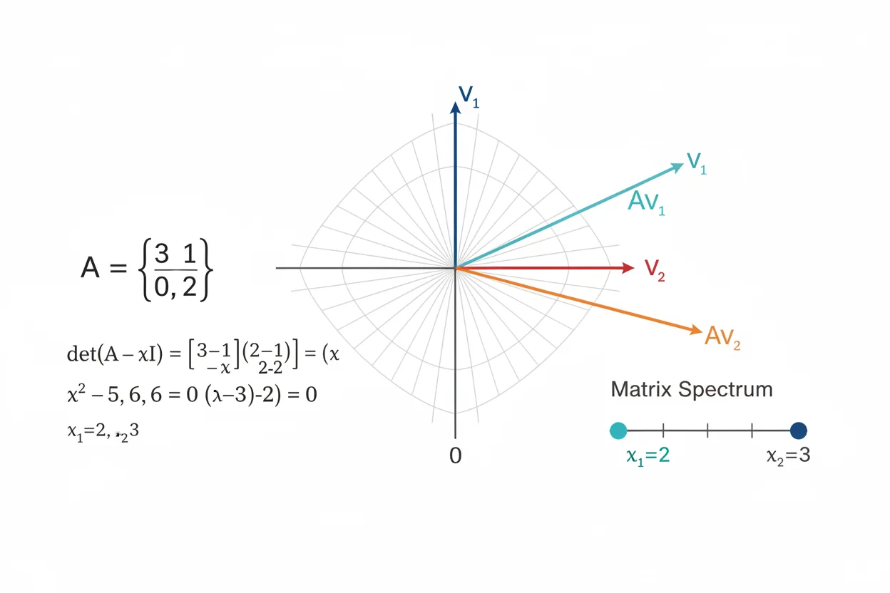
Eigenvalues are the scalar values that describe how a square matrix scales its special eigenvector directions. They are found by solving the characteristic equation det(A − λI) = 0. An n×n matrix has n eigenvalues when algebraic multiplicity is counted over the complex numbers, although some values may repeat and some may not be real. Together, the eigenvalues reveal important structural information about a matrix, including its determinant, trace, invertibility, repeated transformations, and behavior along invariant directions. Distinct eigenvalues usually correspond to linearly independent eigenvectors, while repeated eigenvalues require additional analysis to determine how many independent eigenvectors exist. Diagonal and triangular matrices make eigenvalues easy to identify because their eigenvalues are their diagonal entries. For general matrices, the characteristic polynomial must normally be solved. Eigenvalues are central to linear algebra because they summarize important properties of a transformation in a small collection of scalar values.
What Are Eigenvalues?
Let A be a square matrix.
A scalar λ is an eigenvalue when there is at least one nonzero vector v satisfying:
Av = λv
The corresponding vectors are eigenvectors.
If a matrix has eigenvalues:
λ₁, λ₂, …, λₙ
these values describe how the transformation acts along its eigenvector directions.
For example, an eigenvalue of 4 means the corresponding eigenvectors are multiplied by 4. An eigenvalue of −1 means the corresponding direction is reversed without changing magnitude.
Formula for Eigenvalues
Starting with:
Av = λv
write:
Av − λIv = 0
Then:
(A − λI)v = 0
For a nonzero v to exist:
det(A − λI) = 0
Therefore the eigenvalues are the roots of:
det(A − λI) = 0
The determinant calculation itself follows the rules of a matrix determinant.
Characteristic Polynomial
The expression:
det(A − λI)
is a polynomial in λ called the characteristic polynomial.
For a 2×2 matrix, it is quadratic.
For a 3×3 matrix, it is cubic.
More generally, an n×n matrix has a characteristic polynomial of degree n.
Solving that polynomial produces the eigenvalues, counting repeated roots according to their algebraic multiplicities.
Example: Find All Eigenvalues of a 2×2 Matrix
Let:
A = [ 4 2 ]
[ 1 3 ]
Form:
A − λI = [ 4 − λ 2 ]
[ 1 3 − λ ]
Calculate the determinant:
(4 − λ)(3 − λ) − 2 = 0
Expand:
12 − 7λ + λ² − 2 = 0
λ² − 7λ + 10 = 0
Factor:
(λ − 2)(λ − 5) = 0
Therefore the eigenvalues are:
λ₁ = 2
λ₂ = 5
Checking the Eigenvalues With Trace and Determinant
For the matrix:
A = [ 4 2 ]
[ 1 3 ]
the trace is:
4 + 3 = 7
The eigenvalues sum to:
2 + 5 = 7
The determinant is:
4(3) − 2(1)
= 10
The eigenvalues multiply to:
2 × 5 = 10
Both relationships confirm the calculation.
General 2×2 Eigenvalue Equation
Let:
A = [ a b ]
[ c d ]
Then:
det(A − λI) = 0
becomes:
(a − λ)(d − λ) − bc = 0
Expanding:
λ² − (a + d)λ + (ad − bc) = 0
Therefore:
λ² − trace(A)λ + det(A) = 0
The two eigenvalues are the roots of this quadratic.
Eigenvalues of a Diagonal Matrix
Consider:
A = [ 2 0 0 ]
[ 0 −3 0 ]
[ 0 0 7 ]
The characteristic equation is:
(2 − λ)(−3 − λ)(7 − λ) = 0
Therefore the eigenvalues are:
2, −3, 7
For a diagonal matrix, its diagonal entries are its eigenvalues.
This is one reason diagonal matrix representations are so useful.
Eigenvalues of an Upper-Triangular Matrix
Consider:
A = [ 5 2 1 ]
[ 0 3 4 ]
[ 0 0 −2 ]
Because A is upper triangular, the determinant of A − λI is simply the product of its diagonal entries:
(5 − λ)(3 − λ)(−2 − λ)
Therefore:
λ = 5, 3, −2
The same rule applies to lower-triangular matrices.
Distinct Eigenvalues
Eigenvalues are distinct when no value repeats.
For example:
λ₁ = 1
λ₂ = 4
λ₃ = 7
are three distinct eigenvalues.
A key result is that eigenvectors corresponding to distinct eigenvalues are linearly independent.
This means that if an n×n matrix has n distinct eigenvalues, it automatically has n linearly independent eigenvectors.
That creates a particularly simple structure for the transformation.
Repeated Eigenvalues
Suppose the characteristic polynomial is:
(λ − 3)²(λ + 1)
Then the eigenvalues are:
3, 3, −1
or, listing distinct values:
3 and −1
The eigenvalue 3 has algebraic multiplicity 2.
The eigenvalue −1 has algebraic multiplicity 1.
Repeated eigenvalues are common and require care because algebraic multiplicity does not automatically tell us how many independent eigenvectors exist.
Algebraic Multiplicity
The algebraic multiplicity of an eigenvalue is the number of times it occurs as a root of the characteristic polynomial.
For:
(λ − 2)³(λ + 4) = 0
the eigenvalue:
λ = 2
has algebraic multiplicity 3.
The eigenvalue:
λ = −4
has algebraic multiplicity 1.
The total algebraic multiplicities add to the degree of the characteristic polynomial.
Geometric Multiplicity
The geometric multiplicity of an eigenvalue is the dimension of its eigenspace.
For eigenvalue λ, the eigenspace consists of solutions to:
(A − λI)v = 0
The geometric multiplicity is at least 1 for an actual eigenvalue and cannot exceed its algebraic multiplicity.
Therefore:
1 ≤ geometric multiplicity ≤ algebraic multiplicity
This distinction becomes crucial when deciding whether enough independent eigenvectors exist to form a basis.
Eigenvectors Associated With Eigenvalues
Once an eigenvalue is known, its eigenvector can be found by solving:
(A − λI)v = 0
For example, take:
A = [ 4 2 ]
[ 1 3 ]
and:
λ = 5
Then:
A − 5I = [ −1 2 ]
[ 1 −2 ]
Solve:
−x + 2y = 0
so:
x = 2y
Choose:
y = 1
Then one eigenvector is:
v = (2, 1)
Any nonzero scalar multiple, such as:
(4, 2)
is also an eigenvector for λ = 5.
Why Eigenvectors Can Be Rescaled
Suppose:
Av = λv
If c ≠ 0, then:
A(cv) = cAv
= cλv
= λ(cv)
Therefore every nonzero scalar multiple of an eigenvector is another eigenvector associated with the same eigenvalue.
Eigenvectors therefore represent directions rather than unique vector lengths.
Eigenvalues and Linear Transformations
A matrix represents a linear transformation relative to a chosen basis.
Most input vectors change both direction and length.
Eigenvectors behave differently:
Av = λv
They remain on their original line.
The corresponding eigenvalues determine what happens along those invariant lines.
This makes eigenvalues useful geometric descriptors of an otherwise potentially complicated transformation.
Eigenvalues and Basis Selection
A basis determines the coordinate representation of vectors and matrices, as developed in basis and dimension.
If a matrix has enough linearly independent eigenvectors, those eigenvectors can be used as a basis.
In such coordinates, the transformation becomes especially simple because each basis vector is merely scaled by its corresponding eigenvalue.
Although matrix entries can change under a basis transformation, eigenvalues remain unchanged under similarity.
Eigenvalues and Matrix Multiplication
Repeated application of a matrix relies on matrix multiplication.
If:
Av = λv
then:
A²v = λ²v
and:
A³v = λ³v
In general:
Aⁿv = λⁿv
So powers of a matrix act particularly simply on eigenvectors.
Eigenvalues therefore help analyze long-term behavior when the same linear transformation is applied repeatedly.
Eigenvalues of Aⁿ
If λ is an eigenvalue of A, then:
λⁿ
is an eigenvalue of Aⁿ associated with the same eigenvector.
For example, if:
λ = 2
then for A⁵:
λ⁵ = 2⁵ = 32
is the corresponding eigenvalue.
If:
|λ| > 1
repeated powers grow in magnitude along that eigenvector direction.
If:
|λ| < 1
they shrink toward zero.
If:
λ = −1
the direction alternates sign under repeated applications.
Eigenvalues of an Inverse Matrix
If A is invertible and has nonzero eigenvalues:
λ₁, λ₂, …, λₙ
then the matrix inverse A⁻¹ has eigenvalues:
1/λ₁, 1/λ₂, …, 1/λₙ
This follows from:
Av = λv
which implies:
A⁻¹v = (1/λ)v
A matrix with a zero eigenvalue cannot be inverted.
Eigenvalues and Matrix Invertibility
For a square matrix A, the following statements are equivalent:
0 is not an eigenvalue of A
det(A) ≠ 0
A is invertible
A has full rank
This connects eigenvalues directly with matrix rank and invertibility.
If zero appears among the eigenvalues, at least one nonzero direction is collapsed to zero.
Eigenvalues and Determinants
If the eigenvalues are:
λ₁, λ₂, …, λₙ
counting algebraic multiplicity, then:
det(A) = λ₁λ₂…λₙ
For example, if a 3×3 matrix has eigenvalues:
2, −1, 4
then:
det(A) = 2(−1)(4)
= −8
This provides a quick way to calculate or verify a determinant once the eigenvalues are known.
Eigenvalues and Trace
The trace of a square matrix equals the sum of its eigenvalues, counting algebraic multiplicity:
trace(A) = λ₁ + λ₂ + … + λₙ
For eigenvalues:
2, −1, 4
the trace is:
2 − 1 + 4
= 5
So a corresponding matrix must have diagonal entries summing to 5.
Real and Complex Eigenvalues
A real matrix does not necessarily have only real eigenvalues.
Consider:
A = [ 0 −1 ]
[ 1 0 ]
Its characteristic polynomial is:
λ² + 1
Therefore:
λ = i
and:
λ = −i
These complex eigenvalues reflect rotational behavior.
For real matrices, nonreal complex eigenvalues occur in conjugate pairs.
Symmetric Matrices and Eigenvalues
A real symmetric matrix has particularly strong eigenvalue properties.
All of its eigenvalues are real.
It also has enough mutually orthogonal eigenvectors to form an orthonormal basis.
Orthogonality between vectors can be checked using the dot product:
v₁ · v₂ = 0
for perpendicular eigenvectors.
These properties make symmetric matrices especially important in geometry, optimization, statistics, and applied linear algebra.
Eigenvalues of the Identity Matrix
For the n×n identity matrix I:
Iv = v
for every vector.
Thus:
λ = 1
is the only distinct eigenvalue, with algebraic multiplicity n.
Every nonzero vector is an eigenvector.
Eigenvalues of the Zero Matrix
For the zero matrix:
0v = 0
which can be written:
0v = 0v
So:
λ = 0
is the only eigenvalue.
For an n×n zero matrix, zero has algebraic multiplicity n.
Eigenvalues Under Scalar Multiplication
If A has eigenvalues:
λ₁, λ₂, …, λₙ
then cA has eigenvalues:
cλ₁, cλ₂, …, cλₙ
because:
(cA)v = c(Av)
= cλv
For example, if A has eigenvalues:
2 and 5
then 3A has eigenvalues:
6 and 15
Eigenvalues of A + cI
If λ is an eigenvalue of A, then:
λ + c
is an eigenvalue of:
A + cI
because:
(A + cI)v = Av + cv
= λv + cv
= (λ + c)v
Thus adding a scalar multiple of the identity shifts all eigenvalues by the same amount.
Eigenvalues and Matrix Operations
General matrix operations do not always translate into simple operations on eigenvalues.
For example, it is not generally valid to say that the eigenvalues of A + B are obtained by adding arbitrary eigenvalues of A and B.
Similarly, matrix multiplication is not generally commutative.
Special relationships require additional assumptions, such as shared eigenvectors or compatible matrix structure.
Eigenvalue rules should therefore be applied only when their required conditions hold.
Distinct Eigenvalues and Linear Independence
Suppose:
v₁, v₂, …, vₖ
are eigenvectors corresponding to distinct eigenvalues:
λ₁, λ₂, …, λₖ
Then these eigenvectors are linearly independent.
This result is important because an n×n matrix with n distinct eigenvalues automatically has enough independent eigenvectors to form a basis.
Repeated eigenvalues make the situation less automatic.
Eigenvalues and Systems of Equations
For a candidate eigenvalue λ, finding its eigenvectors requires solving:
(A − λI)v = 0
This is a homogeneous system of linear equations.
Because λ is an eigenvalue:
det(A − λI) = 0
so the coefficient matrix is singular and nonzero solutions exist.
The null space of A − λI is precisely the eigenspace corresponding to λ.
Example With a Repeated Eigenvalue
Consider:
A = [ 3 1 ]
[ 0 3 ]
Then:
A − λI = [ 3 − λ 1 ]
[ 0 3 − λ ]
The characteristic equation is:
(3 − λ)² = 0
Therefore:
λ = 3
with algebraic multiplicity 2.
Now solve:
(A − 3I)v = 0
This gives:
[ 0 1 ] [x] = [0]
[ 0 0 ] [y] [0]
So:
y = 0
while x is free.
The eigenspace consists of nonzero multiples of:
(1, 0)
Thus the geometric multiplicity is 1, even though the algebraic multiplicity is 2.
This example shows why repeated eigenvalues require analysis beyond simply counting roots.
Example With Two Independent Eigenvectors
Consider:
A = [ 3 0 ]
[ 0 3 ]
Again:
λ = 3
has algebraic multiplicity 2.
But now:
A − 3I = [ 0 0 ]
[ 0 0 ]
Every vector satisfies:
(A − 3I)v = 0
So the eigenspace is two-dimensional.
The same repeated eigenvalue can therefore produce very different eigenvector structures depending on the matrix.
Eigenvalues and Long-Term Behavior
Suppose a state evolves by:
xₙ₊₁ = Axₙ
If the initial state contains an eigenvector component with eigenvalue λ, repeated application scales that component by:
λⁿ
This gives several broad behaviors.
When:
|λ| < 1
that component decays.
When:
|λ| > 1
it grows.
When:
λ < 0
its direction alternates.
When:
|λ| = 1
its magnitude may remain unchanged along that eigenvector direction.
This makes eigenvalues useful for studying repeated linear systems.
Eigenvalues and Differential Equations
Systems of differential equations often lead to matrix equations such as:
x′ = Ax
Eigenvalues of A help determine whether solution components grow, decay, oscillate, or remain stable.
For example, positive real eigenvalues often correspond to exponential growth modes, while negative real eigenvalues produce decaying modes in simple linear systems.
Complex eigenvalues can introduce oscillatory behavior.
The full analysis depends on both eigenvalues and eigenvectors.
Eigenvalues Versus Eigenvectors
Eigenvalues are scalars:
λ₁, λ₂, …
Eigenvectors are nonzero vectors:
v₁, v₂, …
connected by:
Avᵢ = λᵢvᵢ
The eigenvalue tells how much the vector is scaled.
The eigenvector identifies the direction that experiences that scaling.
Neither concept fully replaces the other.
Eigenvalues Versus Dot Product
A dot product measures alignment between vectors:
a · b = |a||b| cos θ
Eigenvalues describe invariant scaling under a matrix transformation.
A dot product becomes especially relevant when studying orthogonal eigenvectors of symmetric matrices, but it is not the procedure used to find eigenvalues in general.
Eigenvalues Versus Double Integrals
A double integral accumulates a function over a two-dimensional region.
Eigenvalues arise from square matrices and linear transformations.
Both concepts belong within the broader Calculus & Linear Algebra landscape, but their roles are separate: eigenvalues describe transformation structure, while double integrals measure regional accumulation.
Eigenvalues and Directional Change
A directional derivative measures how a scalar field changes along a selected spatial direction.
Eigenvalues also involve special directions, but the similarity is only conceptual.
For a directional derivative, the scalar describes a rate of change of a function:
Dᵤf = ∇f · u
For eigenvalues, the scalar describes matrix scaling:
Av = λv
These formulas belong to different mathematical operations.
Matrix Representation and Similarity
Two matrices can represent the same linear transformation under different bases.
If:
B = P⁻¹AP
then A and B are similar matrices.
Similar matrices have the same characteristic polynomial and therefore the same eigenvalues.
This reinforces the idea that eigenvalues describe an intrinsic feature of a linear transformation rather than merely the entries appearing in one coordinate representation.
Common Mistakes With Eigenvalues
A frequent mistake is subtracting λ from every matrix entry. In:
A − λI
λ is subtracted only from diagonal entries.
Another error is solving:
det(A) = 0
when the actual task is to find eigenvalues. The correct equation is:
det(A − λI) = 0
Students may also list only distinct roots when algebraic multiplicity matters. If:
(λ − 2)³ = 0
then λ = 2 has multiplicity 3.
Repeated eigenvalues should not be assumed to provide the same number of independent eigenvectors as their algebraic multiplicity.
Another common mistake is assuming all real matrices have real eigenvalues. Rotational matrices can produce complex conjugate eigenvalues.
Finally, checking the sum and product against the trace and determinant is useful, but those checks alone do not prove every individual eigenvalue is correct when more than two values are involved.
Frequently Asked Questions
What are eigenvalues?
Eigenvalues are scalars λ for which a square matrix A has nonzero vectors satisfying:
Av = λv
How do you find eigenvalues?
Solve the characteristic equation:
det(A − λI) = 0
The roots are the eigenvalues.
How many eigenvalues does an n×n matrix have?
Its characteristic polynomial has degree n, so it has n complex roots when algebraic multiplicity is counted. Some roots may repeat.
Can eigenvalues repeat?
Yes. Repeated roots of the characteristic polynomial are repeated eigenvalues.
What is algebraic multiplicity?
It is the number of times an eigenvalue appears as a root of the characteristic polynomial.
What is geometric multiplicity?
It is the dimension of the eigenspace associated with an eigenvalue.
Can eigenvalues be complex?
Yes. A real matrix can have nonreal complex eigenvalues, which occur in conjugate pairs.
What are the eigenvalues of a diagonal matrix?
They are the diagonal entries.
What are the eigenvalues of a triangular matrix?
They are also the diagonal entries.
What does a zero eigenvalue mean?
It means the matrix is singular, has determinant zero, and is not invertible.
How are eigenvalues related to the determinant?
The determinant is the product of the eigenvalues, counting algebraic multiplicities.
How are eigenvalues related to the trace?
The trace is the sum of the eigenvalues, counting algebraic multiplicities.
Do distinct eigenvalues have independent eigenvectors?
Yes. Eigenvectors corresponding to distinct eigenvalues are linearly independent.
Why are eigenvalues useful?
They simplify the analysis of linear transformations, matrix powers, invertibility, repeated systems, stability, and systems of differential equations by identifying invariant scaling behavior.




