


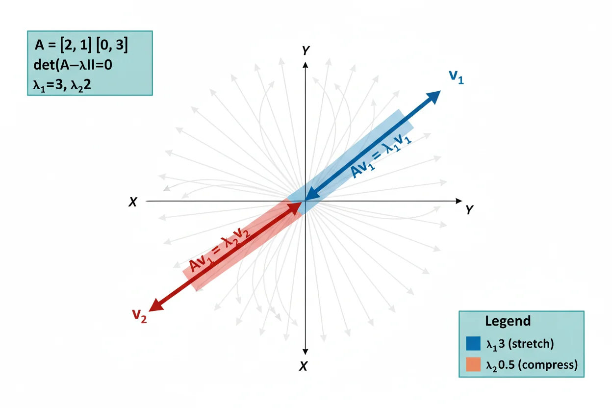
Eigenvectors are the nonzero vectors whose directions remain invariant when a square matrix or linear transformation acts on them. Each eigenvector is paired with an eigenvalue λ through the equation Av = λv. A matrix may have multiple independent eigenvector directions, infinitely many scalar multiples within each eigenspace, or too few independent eigenvectors to form a complete basis. To calculate eigenvectors, first determine the relevant eigenvalues and then solve (A − λI)v = 0 separately for each value of λ. Eigenvectors corresponding to distinct eigenvalues are linearly independent, while repeated eigenvalues require closer examination of their eigenspaces. When enough independent eigenvectors exist, they can form a basis in which the action of the matrix becomes particularly simple. Eigenvectors are therefore central to understanding linear transformations, repeated matrix operations, systems of differential equations, stability, and many matrix-based models. The important distinction is that an individual eigenvector is one nonzero solution, while the broader study of eigenvectors concerns the collection, independence, multiplicity, and structure of these invariant directions.
What Are Eigenvectors?
Let A be an n×n matrix.
The vectors v satisfying:
Av = λv
for some eigenvalue λ and:
v ≠ 0
are eigenvectors of A.
Each eigenvalue can have an entire collection of associated eigenvectors.
If:
v
is one such vector, then:
2v
−5v
0.1v
are also eigenvectors for the same λ, provided the scalar multiplier is nonzero.
Thus eigenvectors naturally occur in families of vectors pointing along the same invariant directions.
Eigenvectors Formula
The defining equation is:
Av = λv
Rearranging:
(A − λI)v = 0
Therefore the general calculation has two stages.
First determine the eigenvalues by solving:
det(A − λI) = 0
Then, for every eigenvalue λᵢ, solve:
(A − λᵢI)v = 0
The nonzero solutions are the eigenvectors associated with λᵢ.
Example: Find the Eigenvectors of a Matrix
Consider:
A = [ 4 1 ]
[ 2 3 ]
The characteristic equation gives the eigenvalues:
λ₁ = 5
and:
λ₂ = 2
We now find the corresponding eigenvectors separately.
Eigenvectors for λ = 5
Form:
A − 5I = [ −1 1 ]
[ 2 −2 ]
Solve:
−x + y = 0
Therefore:
y = x
So the eigenspace consists of vectors:
v = (x, x)
with:
x ≠ 0
A convenient representative is:
v₁ = (1, 1)
Every nonzero multiple of (1, 1) is also an eigenvector for λ = 5.
Eigenvectors for λ = 2
Now form:
A − 2I = [ 2 1 ]
[ 2 1 ]
Solve:
2x + y = 0
Therefore:
y = −2x
So the eigenspace contains:
v = (x, −2x)
for:
x ≠ 0
A convenient representative is:
v₂ = (1, −2)
Thus the matrix has two independent eigendirections represented by:
(1, 1)
and:
(1, −2)
Verifying Both Eigenvectors
Using matrix multiplication:
A(1, 1) = (5, 5)
and:
5(1, 1) = (5, 5)
so:
Av₁ = 5v₁
For the second vector:
A(1, −2) = (2, −4)
and:
2(1, −2) = (2, −4)
so:
Av₂ = 2v₂
Both vectors satisfy the eigenvector equation.
Eigenvectors Belong to Eigenspaces
For each eigenvalue λ, define:
Eλ = null(A − λI)
This set is called the eigenspace associated with λ.
It contains:
- the zero vector,
- every eigenvector associated with λ,
- all linear combinations of those vectors that remain in the null space.
The zero vector belongs to the eigenspace but is not an eigenvector.
For the previous matrix:
E₅ = span{(1, 1)}
and:
E₂ = span{(1, −2)}
Each eigenspace is one-dimensional.
Why There Are Infinitely Many Eigenvectors
Suppose:
v = (1, 1)
is an eigenvector.
Then:
(2, 2)
(3, 3)
(−1, −1)
and every other nonzero scalar multiple also satisfies the same eigenvector relationship.
Therefore even a matrix with only one eigendirection typically has infinitely many eigenvectors.
When discussing the number of eigenvectors, the more useful question is often:
How many linearly independent eigenvectors are there?
rather than how many individual vector multiples exist.
Eigenvectors and Linear Independence
Eigenvectors corresponding to distinct eigenvalues are linearly independent.
Suppose:
Av₁ = λ₁v₁
and:
Av₂ = λ₂v₂
with:
λ₁ ≠ λ₂
Then v₁ and v₂ cannot be scalar multiples of each other.
For the example:
v₁ = (1, 1)
v₂ = (1, −2)
the vectors point in different directions and are linearly independent.
This result extends to any collection of eigenvectors associated with distinct eigenvalues.
Why Linear Independence Matters
In an n-dimensional vector space, n linearly independent vectors form a basis.
The concepts of basis and dimension therefore connect directly with eigenvectors.
If an n×n matrix has n independent eigenvectors:
v₁, v₂, …, vₙ
then every vector in the space can be written as:
x = c₁v₁ + c₂v₂ + … + cₙvₙ
Applying A gives:
Ax = c₁λ₁v₁ + c₂λ₂v₂ + … + cₙλₙvₙ
The transformation acts independently on each eigenvector component.
Eigenvectors and an Eigenbasis
When enough independent eigenvectors exist to form a basis, that basis is called an eigenbasis.
For the matrix:
A = [ 4 1 ]
[ 2 3 ]
the independent eigenvectors:
(1, 1)
and:
(1, −2)
form a basis of the two-dimensional space.
In that basis, the transformation is described simply by the scaling factors:
5 and 2
rather than by the original mixture of matrix entries.
This is a powerful simplification when analyzing repeated transformations.
Distinct Eigenvalues
If an n×n matrix has n distinct eigenvalues, then it automatically has n linearly independent eigenvectors.
For example, a 3×3 matrix with distinct eigenvalues:
2, 5, 9
has at least one eigenvector associated with each value, and those three eigenvectors are linearly independent.
Therefore they form a basis for the three-dimensional vector space.
Distinct eigenvalues provide one of the easiest situations for analyzing eigenvector structure.
Repeated Eigenvalues
Repeated eigenvalues require more care.
Consider:
A = [ 3 1 ]
[ 0 3 ]
The characteristic polynomial is:
(3 − λ)²
so:
λ = 3
has algebraic multiplicity 2.
To find its eigenvectors:
A − 3I = [ 0 1 ]
[ 0 0 ]
The system gives:
y = 0
so all eigenvectors have the form:
(x, 0)
with x ≠ 0.
There is only one independent eigenvector direction:
(1, 0)
Even though the eigenvalue repeats twice, the eigenspace is only one-dimensional.
Algebraic and Geometric Multiplicity
The algebraic multiplicity of an eigenvalue is its multiplicity as a root of the characteristic polynomial.
The geometric multiplicity is the dimension of its eigenspace.
For each eigenvalue:
1 ≤ geometric multiplicity ≤ algebraic multiplicity
In the previous example:
algebraic multiplicity = 2
but:
geometric multiplicity = 1
This mismatch explains why the matrix does not have two independent eigenvectors.
Repeated Eigenvalue With Enough Eigenvectors
Compare the previous matrix with:
A = [ 3 0 ]
[ 0 3 ]
Again:
λ = 3
has algebraic multiplicity 2.
But:
A − 3I = [ 0 0 ]
[ 0 0 ]
Every vector solves the system.
Therefore the eigenspace is two-dimensional.
Two independent choices are:
v₁ = (1, 0)
v₂ = (0, 1)
So the geometric multiplicity is:
2
The same repeated eigenvalue can therefore correspond to very different eigenvector structures.
Eigenvectors of Diagonal Matrices
For a diagonal matrix:
A = [ λ₁ 0 ]
[ 0 λ₂ ]
the coordinate-axis vectors are immediate eigenvectors:
e₁ = (1, 0)
e₂ = (0, 1)
because:
Ae₁ = λ₁e₁
and:
Ae₂ = λ₂e₂
In higher dimensions, the same principle applies.
Diagonal matrices make the independent scaling directions explicit.
Eigenvectors of the Identity Matrix
For the identity matrix:
Iv = v
for every vector v.
Therefore:
Iv = 1v
Every nonzero vector is an eigenvector with:
λ = 1
The eigenspace is the entire vector space.
This is an extreme case in which every direction is invariant.
Eigenvectors of the Zero Matrix
For the zero matrix:
0v = 0
which is:
0v = 0v
Therefore every nonzero vector is an eigenvector associated with:
λ = 0
Again, every direction is invariant in the sense that every vector is collapsed to zero.
Eigenvectors and Linear Transformations
A matrix is one coordinate representation of a linear transformation.
Eigenvectors identify directions that remain invariant under that transformation.
If:
Av = λv
then the transformed vector stays on the line spanned by v.
A transformation may stretch one eigenvector direction, shrink another, and reverse another depending on their corresponding eigenvalues.
These directions reveal the transformation’s internal geometric structure.
Eigenvectors and Matrix Rank
For a given eigenvalue λ:
Eλ = null(A − λI)
The dimension of this eigenspace can be determined using the matrix rank relationship:
nullity(A − λI) = n − rank(A − λI)
That nullity equals the geometric multiplicity.
Therefore matrix rank provides a direct way to determine how many independent eigenvectors belong to a particular eigenvalue.
Eigenvectors and Matrix Determinants
The matrix determinant first enters the process through:
det(A − λI) = 0
This equation identifies the eigenvalues.
Once λ is found, solving:
(A − λI)v = 0
finds the eigenvectors.
The two stages should not be confused: the determinant identifies possible scaling factors, while the null-space calculation identifies the directions associated with them.
Eigenvectors and Matrix Invertibility
If:
λ = 0
is an eigenvalue, then there is some nonzero eigenvector satisfying:
Av = 0
This means A has a nontrivial null space.
Therefore A cannot have a matrix inverse.
If A is invertible, none of its eigenvalues can be zero.
Its eigenvectors are then mapped to nonzero scalar multiples rather than being collapsed completely.
Eigenvectors Under Repeated Matrix Multiplication
Suppose:
Av = λv
Applying A again gives:
A²v = λ²v
More generally:
Aⁿv = λⁿv
Thus repeated matrix action is especially easy to understand along eigenvector directions.
If:
|λ| > 1
that component grows.
If:
|λ| < 1
it shrinks.
If:
λ < 0
its orientation alternates under successive powers.
If:
λ = 1
it remains unchanged.
Eigenvectors and Matrix Operations
Some matrix operations interact cleanly with common eigenvectors.
If the same v satisfies:
Av = λv
and:
Bv = μv
then:
(A + B)v = (λ + μ)v
and:
ABv = λμv
But these relationships require v to be an eigenvector of both A and B.
In general, the eigenvectors of A + B or AB cannot be determined merely by combining arbitrary eigenvectors of the individual matrices.
Orthogonal Eigenvectors
Two vectors are orthogonal when their dot product equals zero:
v₁ · v₂ = 0
For real symmetric matrices, eigenvectors associated with distinct eigenvalues are orthogonal.
For example, consider:
A = [ 2 1 ]
[ 1 2 ]
Its eigenvectors can be represented by:
v₁ = (1, 1)
and:
v₂ = (1, −1)
Their dot product is:
1(1) + 1(−1)
= 0
So they are perpendicular.
Normalized Eigenvectors
An eigenvector can be scaled to have magnitude 1.
For nonzero v:
u = v/|v|
Suppose:
v = (1, 1)
Its magnitude is:
|v| = √2
So a normalized eigenvector is:
u = (1/√2, 1/√2)
Similarly, for:
v = (1, −1)
a normalized form is:
(1/√2, −1/√2)
Normalization is useful when comparing directions or constructing orthonormal bases.
Eigenvectors and Systems of Linear Equations
Finding eigenvectors requires solving:
(A − λI)v = 0
This is a homogeneous system of linear equations.
Because λ is an eigenvalue:
det(A − λI) = 0
so the system must have nontrivial solutions.
Row reduction or direct algebra can be used to express those solutions in terms of free variables.
The free variables determine the basis vectors of the corresponding eigenspace.
Eigenvectors in Systems of Differential Equations
Eigenvectors become especially useful for systems of differential equations written as:
x′ = Ax
Suppose:
Av = λv
Then:
x(t) = e^(λt)v
is a solution mode because:
x′(t) = λe^(λt)v
while:
Ax(t) = e^(λt)Av
= λe^(λt)v
These expressions are equal.
Multiple independent eigenvectors can provide multiple independent solution modes.
Eigenvectors and First-Order Linear Differential Equations
A scalar first-order linear differential equation concerns one dependent variable, while eigenvectors become especially relevant after linear differential equations are organized into vector systems.
For example:
x′ = Ax
turns the coefficients into a matrix.
The eigenvectors of A identify directions in the system’s state space that evolve independently by simple exponential scaling.
This is a system-level extension rather than a replacement for the ordinary first-order solution method.
Eigenvectors and Euler’s Method
The Euler method numerically advances a differential equation using:
xₙ₊₁ = xₙ + hAxₙ
for the linear system:
x′ = Ax
If xₙ lies exactly along an eigenvector v with eigenvalue λ:
Av = λv
then one Euler step gives:
xₙ₊₁ = v + hλv
= (1 + hλ)v
The numerical step remains on the same eigenvector line.
This demonstrates how eigenvectors can clarify the behavior of a numerical method without turning the eigenvector calculation itself into a numerical-integration problem.
Eigenvectors and Long-Term Behavior
Suppose a discrete system evolves as:
xₙ₊₁ = Axₙ
If the starting vector can be decomposed into independent eigenvectors:
x₀ = c₁v₁ + c₂v₂ + …
then after n transformations:
xₙ = c₁λ₁ⁿv₁ + c₂λ₂ⁿv₂ + …
The eigenvalue magnitudes determine which eigenvector components eventually dominate.
A component with:
|λ| > 1
grows, while one with:
|λ| < 1
decays.
This decomposition is one of the most useful interpretations of eigenvectors.
Example: Repeated Transformation
Suppose:
x₀ = 2v₁ + 3v₂
where:
Av₁ = 4v₁
and:
Av₂ = 0.5v₂
After one application:
x₁ = 8v₁ + 1.5v₂
After two:
x₂ = 32v₁ + 0.75v₂
After n applications:
xₙ = 2(4ⁿ)v₁ + 3(0.5ⁿ)v₂
As n grows, the first eigenvector component dominates because:
4ⁿ
grows rapidly while:
0.5ⁿ
approaches zero.
Eigenvectors and Complex Eigenvalues
A real matrix may not have enough real eigenvectors if some eigenvalues are complex.
For example, the rotation matrix:
A = [ 0 −1 ]
[ 1 0 ]
has eigenvalues:
i and −i
Its corresponding eigenvectors require complex components.
Geometrically, a 90-degree rotation has no nonzero real vector that remains on the same real line after the transformation.
Complex eigenvectors allow the eigenvalue framework to extend beyond purely real invariant directions.
Eigenvectors Versus Ordinary Vectors
Every eigenvector is a vector, but not every vector is an eigenvector of a given matrix.
Suppose:
A = [ 4 1 ]
[ 2 3 ]
The vector:
(1, 1)
is an eigenvector because:
A(1, 1) = 5(1, 1)
But:
(1, 0)
is not:
A(1, 0) = (4, 2)
There is no scalar λ satisfying:
(4, 2) = λ(1, 0)
The transformation changes the direction of (1, 0), so it is not an eigenvector.
Eigenvectors Versus Eigenvalues
An eigenvalue is a scalar.
An eigenvector is a nonzero vector.
They are connected by:
Av = λv
The eigenvector gives the invariant direction.
The eigenvalue gives the scaling factor along that direction.
When analyzing an entire matrix, both are usually required for a complete geometric picture.
Eigenvectors Within Calculus and Linear Algebra
Eigenvectors belong primarily to linear algebra, but they interact with calculus through differential equations and dynamical systems.
The broader Calculus & Linear Algebra framework contains both types of ideas.
For comparison, a double integral accumulates a function over a two-dimensional region, while eigenvectors identify invariant transformation directions. The topics can appear in the same advanced mathematical setting without sharing the same core procedure.
Common Eigenvector Mistakes
The most basic mistake is including the zero vector among the eigenvectors. It belongs to every eigenspace but is never itself an eigenvector.
Another error is finding eigenvalues correctly but failing to solve a separate homogeneous system for each eigenvalue.
Students may also list different scalar multiples as though they were independent eigenvector directions. For example:
(1, 2)
and:
(3, 6)
are linearly dependent and represent the same eigendirection.
Repeated eigenvalues require additional care. Their algebraic multiplicity does not automatically equal the number of independent eigenvectors.
It is also incorrect to assume that every n×n matrix has n independent real eigenvectors. Complex eigenvalues or insufficient geometric multiplicity can prevent that.
Finally, every proposed eigenvector should be checked against:
Av = λv
before the calculation is considered complete.
Frequently Asked Questions
What are eigenvectors?
Eigenvectors are nonzero vectors whose directions are preserved under a matrix transformation:
Av = λv
How do you calculate eigenvectors?
Find the eigenvalues first, then solve:
(A − λI)v = 0
for each eigenvalue λ.
Can one eigenvalue have many eigenvectors?
Yes. Every nonzero vector in the corresponding eigenspace is an eigenvector.
Are scalar multiples different eigenvectors?
They are different vector values but represent the same eigenvector direction. Every nonzero scalar multiple remains associated with the same eigenvalue.
What is an eigenspace?
The eigenspace for λ is:
null(A − λI)
It contains all eigenvectors for λ together with the zero vector.
Are eigenvectors from different eigenvalues independent?
Yes. Eigenvectors associated with distinct eigenvalues are linearly independent.
Can repeated eigenvalues have multiple independent eigenvectors?
Yes, but they do not have to. The number of independent eigenvectors is determined by the dimension of the eigenspace.
What is geometric multiplicity?
It is the dimension of an eigenvalue’s eigenspace, which equals the number of independent eigenvector directions associated with that eigenvalue.
What is algebraic multiplicity?
It is the number of times an eigenvalue occurs as a root of the characteristic polynomial.
Can eigenvectors form a basis?
Yes. If an n-dimensional space has n linearly independent eigenvectors, those vectors form an eigenbasis.
Can a matrix have no real eigenvectors?
Yes. A real rotation matrix can have only complex eigenvalues and therefore no nonzero real eigenvectors.
How do you verify eigenvectors?
For each proposed vector v and corresponding eigenvalue λ, calculate both:
Av
and:
λv
If they are identical and v is nonzero, the vector is an eigenvector.




