First-Order Linear Differential Equation: Formula, Rules & Examples

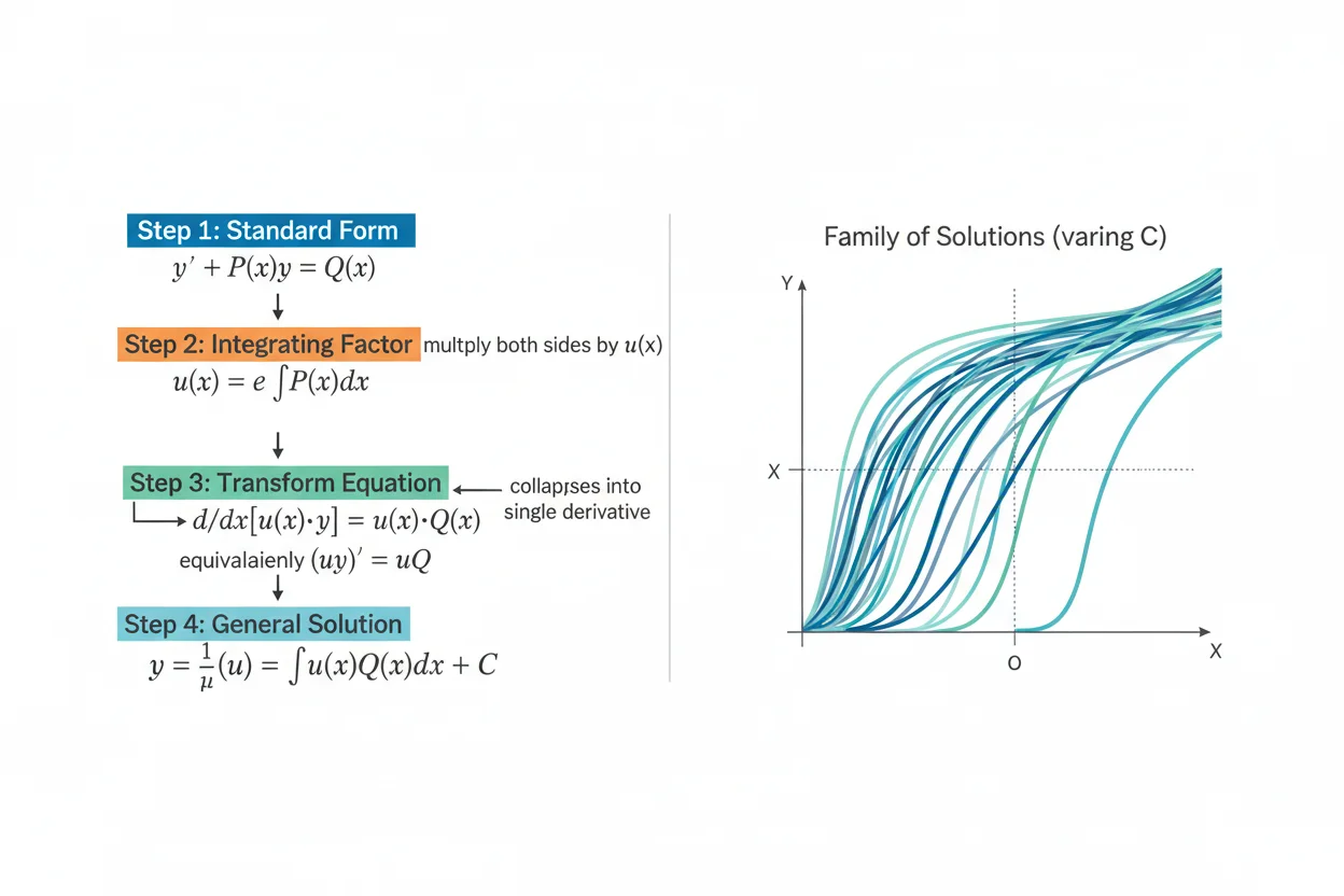
A first-order linear differential equation is an equation that can be written as y′ + P(x)y = Q(x), where y is the unknown function and P(x) and Q(x) depend only on the independent variable. The standard solution method uses an integrating factor μ(x) = e^(∫P(x) dx). Multiplying the equation by this factor transforms the left side into the derivative of a product, (μy)′, so the equation can be integrated directly. The resulting general solution is y = [∫μ(x)Q(x) dx + C]/μ(x). Initial conditions can then determine the constant C and select one particular solution. These equations form an important specialist class within differential equations because a systematic analytic procedure applies whenever the equation is genuinely linear and placed in standard form. Recognizing the coefficients correctly, calculating the integrating factor accurately, and preserving the valid interval of the solution are the key steps.

What Is a First-Order Linear Differential Equation?

The standard form is:

y′ + P(x)y = Q(x)

or equivalently:

dy/dx + P(x)y = Q(x)

It is called first order because the highest derivative is:

y′

It is called linear because y and y′ appear only to the first power and are not multiplied together.

For example:

y′ + 2y = 6

is first-order and linear.

So is:

y′ + x²y = sin x

But:

y′ + y² = x

is nonlinear because y is squared.

Similarly:

yy′ = x

is nonlinear because y and y′ are multiplied together.

The broader derivatives framework explains the rate-of-change quantities appearing here, while the differential equation imposes a relationship that the unknown function must satisfy.

Standard Formula

For:

y′ + P(x)y = Q(x)

define the integrating factor:

μ(x) = e^(∫ P(x) dx)

Multiply the entire differential equation by μ(x):

μy′ + μPy = μQ

The integrating factor is chosen so that:

μ′ = Pμ

Therefore the left side becomes:

(μy)′ = μQ

Integrate:

μy = ∫ μQ dx + C

Finally:

y = [∫ μQ dx + C]/μ

This is the standard first-order linear differential equation solution formula.

Why the Integrating Factor Works

Start with:

y′ + P(x)y = Q(x)

We want the left side to become the derivative of a product.

The product rule gives:

(μy)′ = μy′ + μ′y

After multiplying the original equation by μ:

μy′ + μPy = μQ

For these expressions to match, we require:

μ′y = μPy

so:

μ′ = Pμ

Divide by μ:

μ′/μ = P

Integrate:

∫ μ′/μ dx = ∫ P dx

Therefore:

ln|μ| = ∫ P dx

and a convenient positive integrating factor is:

μ = e^(∫P dx)

The method is therefore built from the product rule operating in reverse.

How to Solve a First-Order Linear Differential Equation

For:

y′ + P(x)y = Q(x)

first make sure the coefficient of y′ is 1.

Then identify:

P(x)

and:

Q(x)

Calculate:

μ(x) = e^(∫P(x) dx)

Multiply every term in the equation by μ.

Rewrite the left side as:

(μy)′

Integrate both sides.

Finally divide by μ and, if an initial condition is given, determine C.

Example: Constant Coefficients

Solve:

y′ + 2y = 6

Here:

P(x) = 2

and:

Q(x) = 6

The integrating factor is:

μ(x) = e^(∫2 dx)

μ(x) = e^(2x)

Multiply the equation by e^(2x):

e^(2x)y′ + 2e^(2x)y = 6e^(2x)

The left side is:

[e^(2x)y]′

Therefore:

[e^(2x)y]′ = 6e^(2x)

Integrate:

e^(2x)y = ∫6e^(2x) dx + C

Since:

∫6e^(2x) dx = 3e^(2x)

we obtain:

e^(2x)y = 3e^(2x) + C

Divide by e^(2x):

y = 3 + Ce^(−2x)

This is the general solution.

Verify the Solution

Take:

y = 3 + Ce^(−2x)

Differentiate:

y′ = −2Ce^(−2x)

Now substitute into:

y′ + 2y

We get:

−2Ce^(−2x) + 2[3 + Ce^(−2x)]

= −2Ce^(−2x) + 6 + 2Ce^(−2x)

= 6

Therefore the function satisfies:

y′ + 2y = 6

Direct substitution is one of the most reliable checks for a differential-equation solution.

Example With an Initial Condition

Solve:

y′ + 2y = 6

subject to:

y(0) = 1

The general solution is:

y = 3 + Ce^(−2x)

Use the initial condition:

1 = 3 + Ce⁰

Since:

e⁰ = 1

we have:

1 = 3 + C

Therefore:

C = −2

The particular solution is:

y = 3 − 2e^(−2x)

Check the initial value:

y(0) = 3 − 2

= 1

Example With a Variable Coefficient

Solve:

y′ + (1/x)y = x²

for:

x > 0

Here:

P(x) = 1/x

The integrating factor is:

μ(x) = e^(∫1/x dx)

On x > 0:

μ(x) = e^(ln x)

μ(x) = x

Multiply the equation by x:

xy′ + y = x³

The left side is:

(xy)′

Therefore:

(xy)′ = x³

Integrate:

xy = x⁴/4 + C

Divide by x:

y = x³/4 + C/x

for:

x > 0

The domain restriction matters because the original equation is undefined at x = 0.

Checking the Variable-Coefficient Example

Start with:

y = x³/4 + C/x

Differentiate:

y′ = 3x²/4 − C/x²

Now calculate:

y′ + y/x

We have:

y/x = x²/4 + C/x²

Therefore:

y′ + y/x = 3x²/4 − C/x² + x²/4 + C/x²

= x²

So the solution satisfies the original equation.

Standard Form Must Come First

Not every linear equation is initially written as:

y′ + P(x)y = Q(x)

For example:

2y′ + 4y = 10

The coefficient of y′ is 2.

Divide the entire equation by 2:

y′ + 2y = 5

Now:

P(x) = 2

Q(x) = 5

and the integrating factor can be found correctly.

Using P = 4 directly would produce the wrong integrating factor because the equation was not yet in standard form.

Example Requiring Standardization

Solve:

xy′ + 2y = x³

for:

x ≠ 0

Divide by x:

y′ + (2/x)y = x²

Now:

P(x) = 2/x

The integrating factor is:

μ(x) = e^(∫2/x dx)

On any interval that does not cross zero:

μ(x) = x²

Multiply through:

x²y′ + 2xy = x⁴

The left side is:

(x²y)′

Therefore:

(x²y)′ = x⁴

Integrate:

x²y = x⁵/5 + C

So:

y = x³/5 + C/x²

The solution is valid on intervals that do not include x = 0.

What Makes the Equation Linear?

A first-order equation is linear in y when it can be expressed as:

a₁(x)y′ + a₀(x)y = g(x)

where the coefficients depend only on x.

After dividing by a₁(x), assuming it is nonzero on the interval:

y′ + P(x)y = Q(x)

The following are linear:

y′ + xy = eˣ

(1 + x²)y′ − 3y = x

y′ − 4y = 0

The following are nonlinear:

y′ + y² = x

y′ = sin(y)

yy′ + x = 0

The key is the way the unknown function y and its derivative appear.

Homogeneous First-Order Linear Equations

If:

Q(x) = 0

the equation becomes:

y′ + P(x)y = 0

This is a homogeneous first-order linear equation.

The solution can be written:

y = Ce^[−∫P(x) dx]

For example:

y′ + 3y = 0

has:

P(x) = 3

so:

y = Ce^(−3x)

This result also follows from separation of variables because the homogeneous first-order linear equation is separable.

Nonhomogeneous First-Order Linear Equations

If:

Q(x) ≠ 0

the equation is nonhomogeneous:

y′ + P(x)y = Q(x)

The general solution contains two conceptual parts:

y = homogeneous part + particular part

The arbitrary constant appears in the homogeneous component.

For:

y′ + 2y = 6

we found:

y = Ce^(−2x) + 3

Here:

Ce^(−2x)

solves the homogeneous equation:

y′ + 2y = 0

while:

3

is one particular solution of the full equation.

Integrating Factor Formula

The integrating factor is:

μ(x) = e^(∫P(x) dx)

The constant of integration normally does not need to be included when calculating μ.

For example:

e^(∫P dx + C)

can be written as:

e^C e^(∫P dx)

The factor e^C is merely a nonzero constant multiplier.

Multiplying an integrating factor by a nonzero constant does not change the resulting solution method.

Example With P(x) = −1

Solve:

y′ − y = eˣ

Here:

P(x) = −1

so:

μ(x) = e^(∫−1 dx)

= e^(−x)

Multiply:

e^(−x)y′ − e^(−x)y = 1

Thus:

[e^(−x)y]′ = 1

Integrate:

e^(−x)y = x + C

Therefore:

y = eˣ(x + C)

Verify the Example

Take:

y = eˣ(x + C)

Differentiate using the product rule:

y′ = eˣ(x + C) + eˣ

= eˣ(x + C + 1)

Then:

y′ − y = eˣ(x + C + 1) − eˣ(x + C)

= eˣ

The solution is correct.

Example With an Integrating Factor Containing x²

Solve:

y′ + 2xy = x

Here:

P(x) = 2x

The integrating factor is:

μ(x) = e^(∫2x dx)

= e^(x²)

Multiply the equation:

e^(x²)y′ + 2xe^(x²)y = xe^(x²)

The left side becomes:

[e^(x²)y]′

Therefore:

[e^(x²)y]′ = xe^(x²)

Integrate:

e^(x²)y = ∫xe^(x²) dx + C

Use the structure recognized in integration by substitution.

Since:

∫xe^(x²) dx = (1/2)e^(x²)

we get:

e^(x²)y = (1/2)e^(x²) + C

Therefore:

y = 1/2 + Ce^(−x²)

When Integration by Parts Appears

The integrating-factor method always reduces the equation to an integral:

∫ μ(x)Q(x) dx

That integral may be simple, or it may require another technique.

For example, an expression involving a polynomial multiplied by an exponential function may lead naturally to integration by parts.

The integrating-factor procedure and the integration technique are separate decisions: the first determines the structure of the solution, while the second evaluates the resulting integral.

Relation to Indefinite Integrals

The general solution contains an indefinite integral:

∫ μ(x)Q(x) dx

This is why the arbitrary constant C appears.

Conceptually, solving the equation reverses a differentiation relationship to recover a family of possible functions.

The wider theory of integrals explains this antiderivative process independently of the differential-equation classification.

Initial Conditions and Particular Solutions

Suppose a general solution is:

y = 4 + Ce^(−x)

and the condition is:

y(0) = 7

Then:

7 = 4 + C

so:

C = 3

The particular solution is:

y = 4 + 3e^(−x)

A first-order equation generally needs one appropriate initial condition to determine the single arbitrary constant in its general solution.

Initial Condition at x = a

If:

y(a) = y₀

substitute x = a and y = y₀ into the general solution.

For example:

y = 2 + Ce^(−3x)

with:

y(1) = 5

gives:

5 = 2 + Ce^(−3)

Therefore:

C = 3e³

So:

y = 2 + 3e³e^(−3x)

which can also be written:

y = 2 + 3e^[−3(x − 1)]

Both forms represent the same particular solution.

Integrating Factor and the Product Rule

The entire method depends on recognizing:

μy′ + μ′y = (μy)′

This is why the coefficient P(x) is used to construct μ.

The method is not simply multiplication by an arbitrary function. The integrating factor is chosen specifically so that:

μ′ = Pμ

Once this occurs, two separate terms collapse into one derivative.

This structural simplification is the central idea of the method.

First-Order Linear Equation Versus Separable Equation

A separable equation can be rearranged into:

g(y)dy = h(x)dx

A first-order linear equation has form:

y′ + P(x)y = Q(x)

Some equations belong to both categories.

For example:

y′ + 2y = 0

can be written:

y′ = −2y

and is separable.

However:

y′ + 2y = x

is linear but is not directly separable into a product of a function of y and a function of x.

The integrating-factor method handles both homogeneous and nonhomogeneous linear equations systematically.

First-Order Linear Equation Versus Euler Method

The Euler method produces numerical approximations:

y₀, y₁, y₂, …

from an initial condition.

The integrating-factor method seeks an analytic expression such as:

y = 3 − 2e^(−2x)

for the entire solution on an interval.

When a first-order linear equation has integrals that can be evaluated conveniently, the analytic method is usually preferable for an exact formula.

Euler’s method remains useful for numerical approximation, comparisons, or equations for which symbolic expressions become impractical.

Euler Check of an Exact Linear Solution

Take:

y′ + 2y = 6

with:

y(0) = 1

The exact solution is:

y = 3 − 2e^(−2x)

Rearrange the differential equation:

y′ = 6 − 2y

Using h = 0.1, Euler’s first step gives:

y₁ = 1 + 0.1[6 − 2(1)]

= 1 + 0.4

= 1.4

The exact value at x = 0.1 is:

y(0.1) = 3 − 2e^(−0.2)

≈ 1.36254

Euler’s estimate is close but not exact.

This illustrates the distinction between a numerical update and the integrating-factor solution.

First-Order Linear Equations and the Fundamental Theorem

After multiplying by the integrating factor:

(μy)′ = μQ

integration gives:

μ(x)y(x) − μ(a)y(a) = ∫ₐˣ μ(t)Q(t) dt

This form follows directly from the Fundamental Theorem of Calculus.

For an initial condition y(a) = y₀:

μ(x)y(x) = μ(a)y₀ + ∫ₐˣ μ(t)Q(t) dt

Therefore:

y(x) = [μ(a)y₀ + ∫ₐˣ μ(t)Q(t) dt]/μ(x)

This definite-integral form incorporates the initial condition without first introducing an arbitrary constant.

Definite-Integral Solution Form

For:

y′ + P(x)y = Q(x)

and:

y(a) = y₀

define:

μ(x) = e^(∫ P(x) dx)

using any convenient antiderivative in the exponent.

Then:

y(x) = [μ(a)y₀ + ∫ₐˣ μ(t)Q(t) dt]/μ(x)

The definite integral accumulates the forcing contribution μQ from the initial point to x.

This form is particularly useful when an initial condition is specified from the beginning.

Existence on an Interval

The coefficients P(x) and Q(x) determine where the equation is well behaved.

If P and Q are continuous on an interval containing the initial point, the standard first-order linear initial-value problem has a well-behaved unique solution throughout that interval.

This is one reason continuity matters when interpreting the formula.

If a coefficient contains:

1/x

then x = 0 divides the real line into separate intervals:

x < 0

and:

x > 0

A solution derived on one interval should not automatically be extended through the singular point.

Example With a Singular Coefficient

Consider:

y′ + (1/x)y = 0

The equation is undefined at:

x = 0

For x > 0:

μ = x

and:

(xy)′ = 0

Therefore:

xy = C

so:

y = C/x

The same formula may also hold on x < 0 with a separately determined constant, but a single initial-value solution does not pass through x = 0 because the differential equation itself is undefined there.

First-Order Linear Equations and Limits

Expressions involving coefficients or solutions may need local analysis near endpoints or singular points.

The theory of a limit can describe what a solution approaches even when the differential equation is not defined at the limiting point.

However, possessing a finite limit does not automatically mean the equation or its solution can be extended through that point while preserving the same differential relationship.

Domain analysis must therefore accompany the algebra.

First-Order Linear Equations and Differentials

The equation:

dy/dx + P(x)y = Q(x)

uses derivative notation, while differentials help express the local relation between changes.

After multiplication by μ:

d(μy)/dx = μQ

which can be written informally as:

d(μy) = μQ dx

Integrating both sides gives:

μy = ∫μQ dx + C

This notation highlights the reversal from differentiation to integration.

First-Order Linear Equations and Gradients

A first-order linear ordinary differential equation involves one independent variable and therefore does not require a gradient for its basic solution.

Gradients belong to multivariable scalar functions and combine several partial derivatives.

The concepts meet in more advanced differential-equation systems and partial differential equations, but the integrating-factor method here remains a one-variable technique.

Keeping that distinction clear prevents multivariable tools from being inserted unnecessarily into an ordinary first-order problem.

Eigenvectors in Linear Differential Systems

A scalar first-order linear equation has one dependent variable.

A system can instead take matrix form:

x′ = Ax

In that setting, eigenvectors of A can identify independent solution directions.

If:

Av = λv

then:

x(t) = e^(λt)v

provides a solution mode.

An individual eigenvector therefore becomes important for systems, whereas the integrating factor directly handles the scalar first-order equation:

y′ + P(x)y = Q(x)

These methods solve related but distinct forms of linear differential equations.

First-Order Linear Differential Equations Within Calculus

The topic sits naturally within the broader Calculus & Linear Algebra framework because solving the equation combines differentiation, integration, function behavior, and, in systems, linear algebra.

For a scalar equation, the essential sequence is:

standardize → find μ → multiply → recognize product derivative → integrate → apply condition

Following this structure prevents most procedural errors.

Common Mistakes

The most frequent mistake is calculating the integrating factor before putting the equation into standard form.

For:

2y′ + 6y = x

you must first divide by 2:

y′ + 3y = x/2

Only then is:

P(x) = 3

Another error is multiplying only some terms by μ. Every term in the equation must be multiplied by the integrating factor.

Students may also fail to recognize that:

μy′ + μ′y

is:

(μy)′

and instead integrate the two terms independently in an unnecessarily complicated way.

The sign in:

μ = e^(∫P dx)

must come directly from P(x). A negative P produces a negative exponent when its integral is negative.

Another common mistake is forgetting C when an indefinite integral is used.

Finally, the equation’s domain must be preserved. Dividing by a coefficient that becomes zero can split the problem into separate intervals, and a solution formula should not be extended automatically across a singularity.

Frequently Asked Questions

What is a first-order linear differential equation?

It is an equation that can be written as:

y′ + P(x)y = Q(x)

where y and y′ appear linearly.

Why is it called first order?

Because the highest derivative in the equation is the first derivative y′.

Why is it called linear?

Because y and y′ appear only to the first power, are not multiplied together, and have coefficients depending only on the independent variable.

What is the integrating factor formula?

For:

y′ + P(x)y = Q(x)

the integrating factor is:

μ(x) = e^(∫P(x) dx)

What is the general solution formula?

After finding μ:

y = [∫μ(x)Q(x) dx + C]/μ(x)

Do I need to put the equation in standard form first?

Yes. The coefficient of y′ should be 1 before identifying P(x) and calculating the integrating factor.

Why does the integrating factor work?

It makes the left side equal to a product derivative:

μy′ + μ′y = (μy)′

because μ is chosen so that:

μ′ = Pμ

Is every first-order equation linear?

No. Equations containing terms such as y², yy′, or nonlinear functions of y are generally nonlinear.

Is every first-order linear equation separable?

No. Homogeneous equations of the form y′ + P(x)y = 0 are separable, but a general nonhomogeneous linear equation need not be.

How do you use an initial condition?

First find the general solution, then substitute the given x- and y-values to determine C. Alternatively, use the definite-integral form incorporating the initial condition directly.

Can the integrating factor method give an exact solution?

Yes, it provides an analytic representation. Whether that representation can be simplified into elementary functions depends on the integral ∫μQ dx.

What is the difference between this method and Euler’s method?

The integrating-factor method derives an analytic solution for a first-order linear equation. Euler’s method approximates an initial-value solution numerically through discrete tangent steps.

How do you check the final solution?

Differentiate the proposed y(x), substitute y and y′ into the original differential equation, and verify that both sides agree. Also check any given initial condition.